Plotting vector fields

First, though, we will generate a standard Gaussian random field so that we have a nice gradient:

# Generate a vector field with a gradient
from scipy.ndimage.filters import gaussian_filter
x = np.arange(0,10,0.5)
y = np.arange(0,10,0.5)
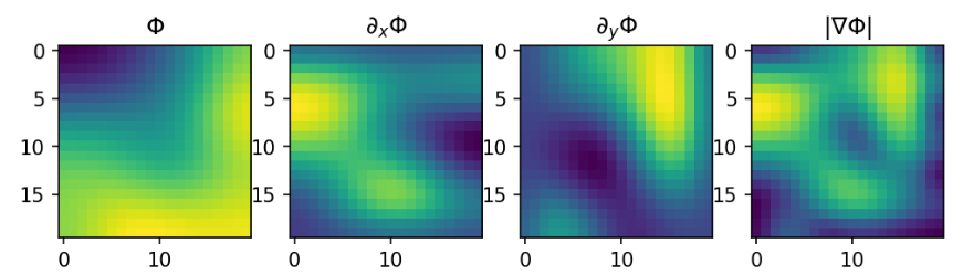
phi = gaussian_filter(np.random.uniform(size=(20,20)), sigma=5)
plt.subplot(141)
plt.imshow(phi, interpolation='none')
plt.title(r'$\Phi$')
plt.subplot(142)
plt.imshow(np.gradient(phi)[0], interpolation='none')
plt.title(r'$\partial_x\Phi$')
plt.subplot(143)
plt.title(r'$\partial_y\Phi$')
plt.imshow(np.gradient(phi)[1], interpolation='none')
plt.subplot(144)
plt.title(r'$\|\nabla \Phi\|$')
plt.imshow(np.linalg.norm(np.gradient(phi), axis=0), interpolation='none')
plt.gcf().set_size_inches(8,4)

Following is the output of the preceding code:

Let's take look...