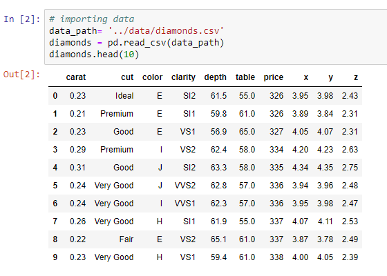
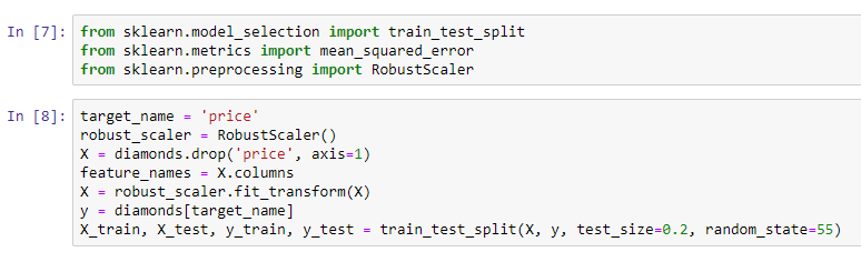
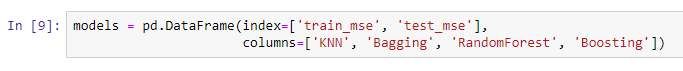
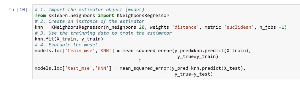
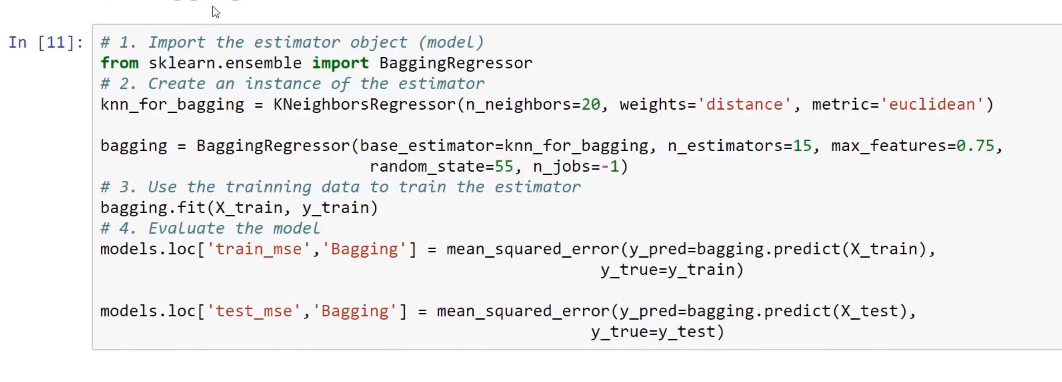
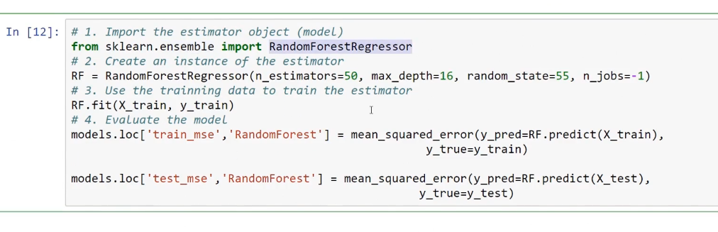
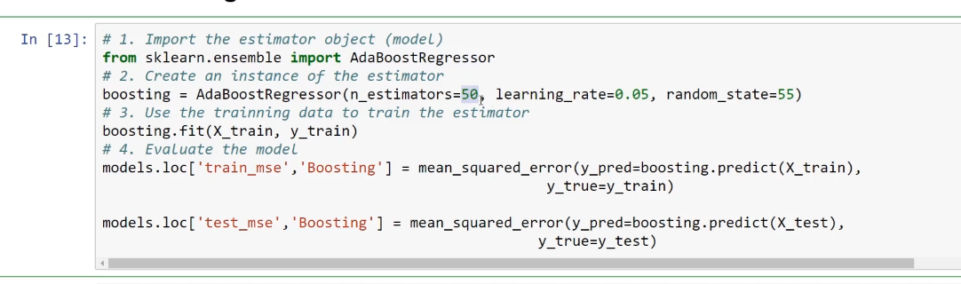
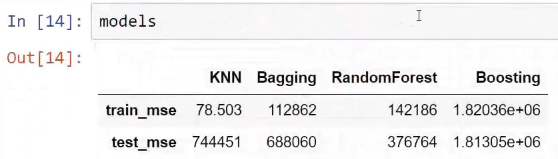
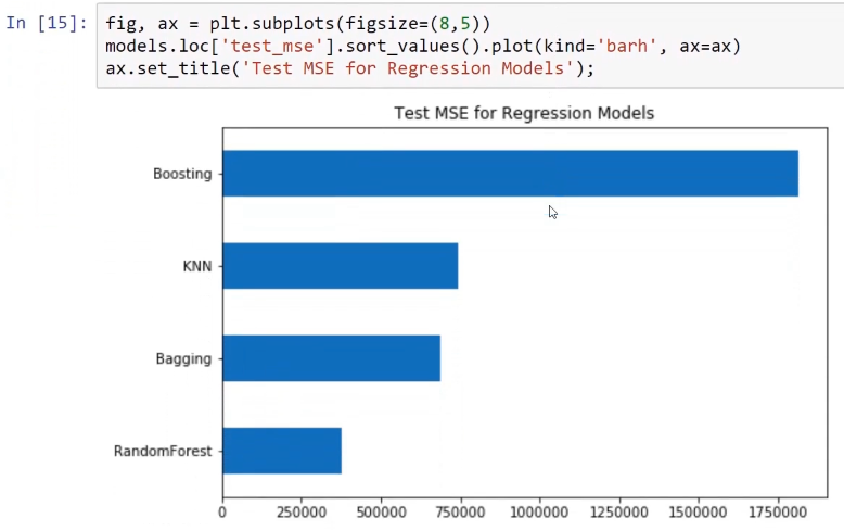
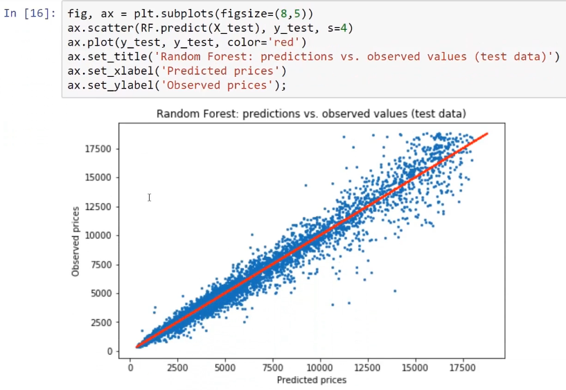
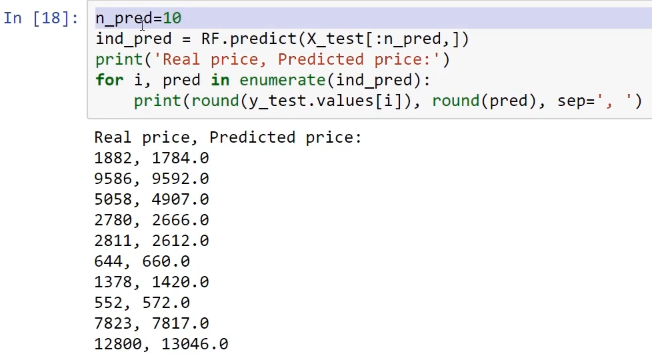
Regarding regression, we will train these different models and later compare their results. In order to test all of these models, we will need a sample dataset. We are going to use this in order to implement these methods on the given dataset and see how this helps us with the performance of our models.
-
Book Overview & Buying
-
Table Of Contents

Mastering Predictive Analytics with scikit-learn and TensorFlow
By :
Mastering Predictive Analytics with scikit-learn and TensorFlow
By:
Overview of this book
Python is a programming language that provides a wide range of features that can be used in the field of data science. Mastering Predictive Analytics with scikit-learn and TensorFlow covers various implementations of ensemble methods, how they are used with real-world datasets, and how they improve prediction accuracy in classification and regression problems.
This book starts with ensemble methods and their features. You will see that scikit-learn provides tools for choosing hyperparameters for models. As you make your way through the book, you will cover the nitty-gritty of predictive analytics and explore its features and characteristics. You will also be introduced to artificial neural networks and TensorFlow, and how it is used to create neural networks. In the final chapter, you will explore factors such as computational power, along with improvement methods and software enhancements for efficient predictive analytics.
By the end of this book, you will be well-versed in using deep neural networks to solve common problems in big data analysis.
Table of Contents (7 chapters)
Preface
 Free Chapter
Ensemble Methods for Regression and Classification
Cross-validation and Parameter Tuning
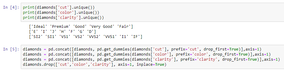
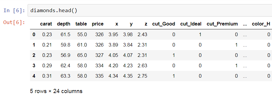
Working with Features
Introduction to Artificial Neural Networks and TensorFlow
Predictive Analytics with TensorFlow and Deep Neural Networks
Other Books You May Enjoy