Bollinger Bands are a statistical method, used for deriving information about the prices and volatility of a certain asset over time. To obtain the Bollinger Bands, we need to calculate the moving average and standard deviation of the time series (prices), using a specified window (typically, 20 days). Then, we set the upper/lower bands at K times (typically, 2) the moving standard deviation above/below the moving average.

The interpretation of the bands is quite sample: the bands widen with an increase in volatility and contract with a decrease in volatility.

In this recipe, we build a simple trading strategy, with the following rules:

• Buy when the price crosses the lower Bollinger Band upwards.
• Sell (only if stocks are in possession) when the price crosses the upper Bollinger Band downward.
• All-in strategy—when creating a buy order, buy as many shares as possible.
• Short selling is not allowed.

We evaluate the strategy on Microsoft's stock in 2018. Additionally, we set the commission to be equal to 0.1%.

Execute the following steps to backtest a strategy based on the Bollinger Bands.

1. Import the libraries:

import backtrader as bt
import datetime
import pandas as pd

2. The template of the strategy is presented:

class BBand_Strategy(bt.Strategy):
    params = (('period', 20), 
              ('devfactor', 2.0),)

    def __init__(self):
        # some code
        
    def log(self, txt):
        # some code

    def notify_order(self, order):
        # some code

    def notify_trade(self, trade):
        # some code

    def next_open(self):
        # some code

The __init__ block is defined as:

    def __init__(self):
        # keep track of close price in the series
        self.data_close = self.datas[0].close
        self.data_open = self.datas[0].open

        # keep track of pending orders/buy price/buy commission
        self.order = None
        self.price = None
        self.comm = None

        # add Bollinger Bands indicator and track the buy/sell signals
        self.b_band = bt.ind.BollingerBands(self.datas[0], 
                                            period=self.p.period, 
                                            devfactor=self.p.devfactor)
        self.buy_signal = bt.ind.CrossOver(self.datas[0], 
                                           self.b_band.lines.bot)
        self.sell_signal = bt.ind.CrossOver(self.datas[0], 
                                            self.b_band.lines.top)

The log block is defined as:

def log(self, txt):
        dt = self.datas[0].datetime.date(0).isoformat()
        print(f'{dt}, {txt}')

The notify_order block is defined as:

 def notify_order(self, order):
        if order.status in [order.Submitted, order.Accepted]:
            return

        if order.status in [order.Completed]:
            if order.isbuy():
                self.log(
                    f'BUY EXECUTED --- Price: {order.executed.price:.2f}, Cost: {order.executed.value:.2f}, Commission: {order.executed.comm:.2f}'
                )
                self.price = order.executed.price
                self.comm = order.executed.comm
            else:
                self.log(
                    f'SELL EXECUTED --- Price: {order.executed.price:.2f}, Cost: {order.executed.value:.2f}, Commission: {order.executed.comm:.2f}'
                )

        elif order.status in [order.Canceled, order.Margin, 
                              order.Rejected]:
            self.log('Order Failed')

        self.order = None

The notify_trade block is defined as:

def notify_trade(self, trade):
        if not trade.isclosed:
            return

        self.log(f'OPERATION RESULT --- Gross: {trade.pnl:.2f}, Net: {trade.pnlcomm:.2f}')

The next_open block is defined as:

def next_open(self):
        if not self.position:
            if self.buy_signal > 0:
                size = int(self.broker.getcash() / self.datas[0].open)
                self.log(f'BUY CREATED --- Size: {size}, Cash: {self.broker.getcash():.2f}, Open: {self.data_open[0]}, Close: {self.data_close[0]}')
                self.buy(size=size)
        else: 
            if self.sell_signal < 0:
                self.log(f'SELL CREATED --- Size: {self.position.size}')
                self.sell(size=self.position.size)

3. Download the data:

data = bt.feeds.YahooFinanceData(
    dataname='MSFT',
    fromdate=datetime.datetime(2018, 1, 1),
    todate=datetime.datetime(2018, 12, 31)
)

4. Set up the backtest:

cerebro = bt.Cerebro(stdstats = False, cheat_on_open=True)

cerebro.addstrategy(BBand_Strategy)
cerebro.adddata(data)
cerebro.broker.setcash(10000.0)
cerebro.broker.setcommission(commission=0.001)
cerebro.addobserver(bt.observers.BuySell)
cerebro.addobserver(bt.observers.Value)
cerebro.addanalyzer(bt.analyzers.Returns, _name='returns')
cerebro.addanalyzer(bt.analyzers.TimeReturn, _name='time_return')

5. Run the backtest:

print('Starting Portfolio Value: %.2f' % cerebro.broker.getvalue())
backtest_result = cerebro.run()
print('Final Portfolio Value: %.2f' % cerebro.broker.getvalue())

6. Plot the results:

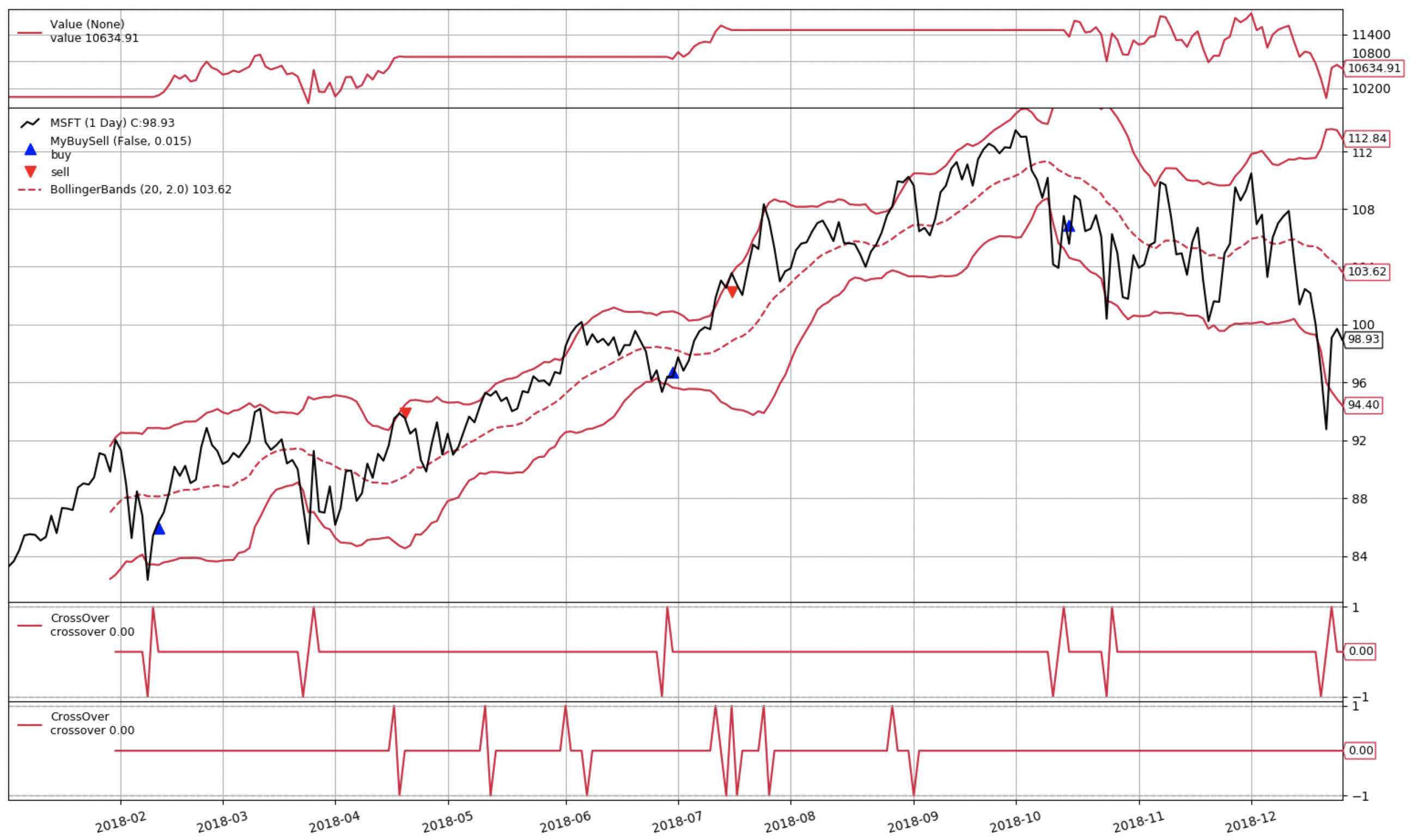
cerebro.plot(iplot=True, volume=False)

The resulting graph is presented below:

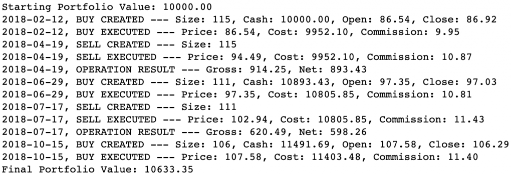
The log is presented below:

We can see that the strategy managed to make money, even after accounting for commission costs. We now turn to an inspection of the analyzers.

7. Run the following code to investigate different returns metrics:

print(backtest_result[0].analyzers.returns.get_analysis())

The output of the preceding line is as follows:

OrderedDict([('rtot', 0.06155731237239935), 
             ('ravg', 0.00024622924948959743), 
             ('rnorm', 0.06401530037885826), 
             ('rnorm100', 6.401530037885826)])

8. Create a plot of daily portfolio returns:

returns_dict = backtest_result[0].analyzers.time_return.get_analysis()
returns_df = pd.DataFrame(list(returns_dict.items()), 
                          columns = ['report_date', 'return']) \
               .set_index('report_date')
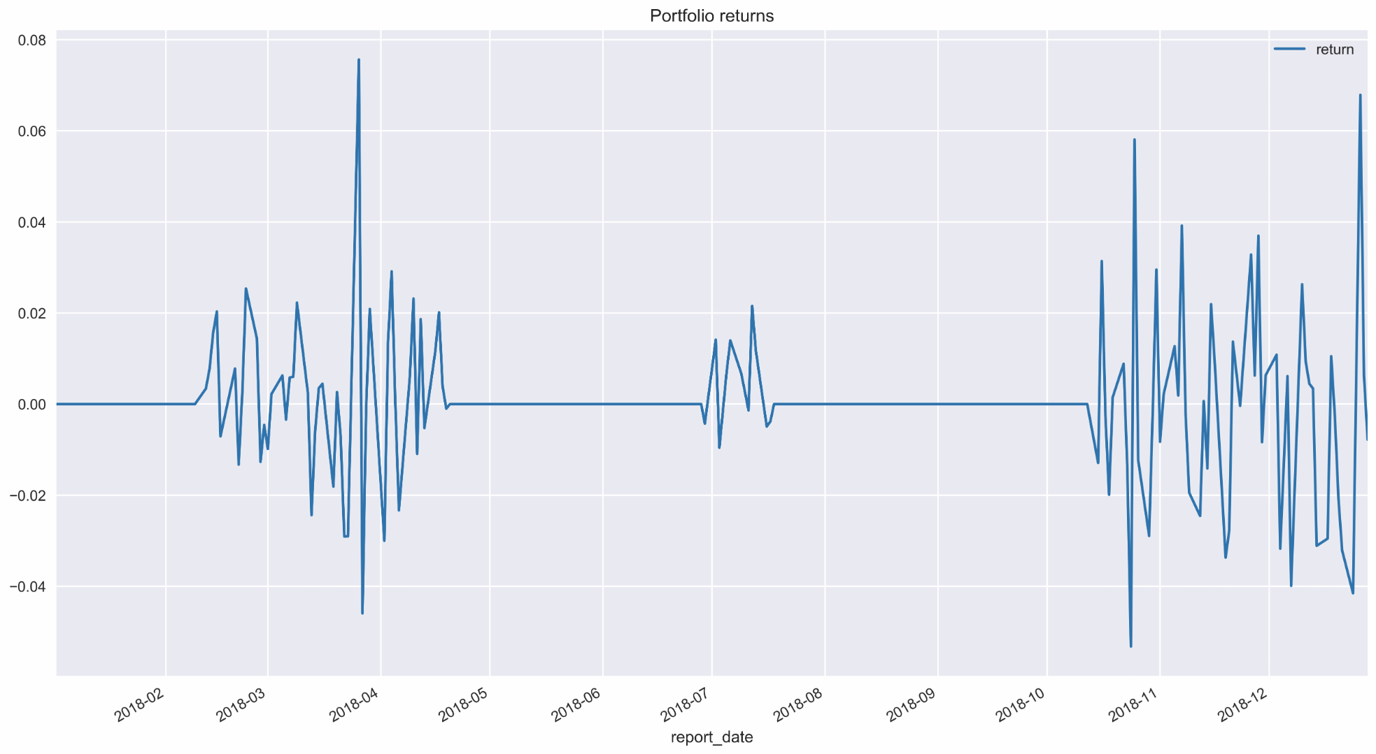
returns_df.plot(title='Portfolio returns')

Running the code results in the following plot:

The flat lines represent periods when we have no open positions.

There are a lot of similarities between the code used for creating the Bollinger Bands-based strategy and that used in the previous recipe. That is why we only discuss the novelties, and refer you to the Backtesting a strategy based on simple moving average recipe for more details.

As we were going all-in in this strategy, we had to use a method called cheat_on_open. This means that we calculated the signals on day t's close price, but calculated the number of shares we wanted to buy based on day t+1's open price. To do so, we had to set cheat_on_open=True when creating the bt.Cerebro object. As a result, we also defined a next_open method instead of next within the Strategy class. This clearly indicated to Cerebro that we were cheating-on-open. Before creating a potential buy order, we calculated size = int(self.broker.getcash() / self.datas[0].open), which is the maximum number of shares we could buy (the open price comes from day t+1). The last novelty was that we also added commission directly to Cerebro by using cerebro.broker.setcommission(commission=0.001).

When calculating the buy/sell signals based on the Bollinger Bands, we used the CrossOver indicator. It returned the following:

• 1 if the first data (price) crossed the second data (indicator) upward
• -1 if the first data (price) crossed the second data (indicator) downward

The last addition included utilizing analyzers—backtrader objects that help to evaluate what is happening with the portfolio. In the following example, we used two analyzers:

• Returns: A collection of different logarithmic returns, calculated on the entire timeframe: total compound return, the average return over the entire period, and the annualized return.
• TimeReturn: A collection of returns over time (using a provided time-frame, in this case, daily data).