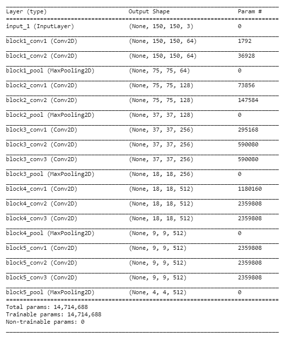
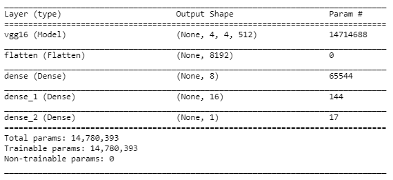
Transfer learning helps us solve a new problem using fewer examples by using information gained from solving other related tasks. It is a technique where we reuse a learned model trained on a different dataset to solve a similar but different problem. In transfer learning, we extend the learning of a pre-trained model in our network and build a new model to solve a new learning problem. The keras library in R provides many pre-trained models; we will be using one such model called as VGG16 to train our network.

library(keras)

train_path <- "dogs_cats_small/train/"
test_path <- "dogs_cats_small/test/"
validation_path <- "dogs_cats_small/validation/"

We have set the paths of our dataset.

1. We start by defining a generator for the training and testing data. We will use these generators while loading data into our environment and perform real-time data augmentation:

# train generator
train_augmentor = image_data_generator(
 rescale = 1/255,
 rotation_range = 300,
 width_shift_range = 0.15,
 height_shift_range = 0.15,
 shear_range = 0.2,
 zoom_range = 0.2,
 horizontal_flip = TRUE,
 fill_mode = "nearest"
)

# test generator
test_augmentor <- image_data_generator(rescale = 1/255)

Now let's load the training, testing, and validation data into our environment:

# load train data
train_data <- flow_images_from_directory(
 train_path,
 train_augmentor,
 target_size = c(150, 150),
 batch_size = 20,
 class_mode = "binary")

# load test data
test_data <- test_generator <- flow_images_from_directory(
 test_path,
 test_augmentor,
 target_size = c(150, 150),
 batch_size = 20,
 class_mode = "binary")

# load validation data
validation_data <- flow_images_from_directory(
 validation_path,
 test_augmentor,
 target_size = c(150, 150),
 batch_size = 20,
 class_mode = "binary"
)

We can print the shape of the rescaled image using the following code:

train_data$image_shape

2. After loading our data, let's instantiate a pre-trained VGG16 model. Going further, we will refer to this model as the base model:

pre_trained_base <- application_vgg16(
 weights = "imagenet",
 include_top = FALSE,
 input_shape = c(150, 150, 3)
)

Let's now take a look at the summary of the base model:

summary(pre_trained_base)

Here is the description of the base model:

After instantiating the base model, we add dense layers to it and build a holistic model:

model_with_pretrained <- keras_model_sequential() %>% 
 pre_trained_base %>% 
 layer_flatten() %>% 
 layer_dense(units = 8, activation = "relu") %>%
 layer_dense(units = 16, activation = "relu") %>%
 layer_dense(units = 1, activation = "sigmoid")

Now we visualize the summary of the model:

summary(model_with_pretrained)

The screenshot shows a summary of the holistic model:

We can print the number of trainable kernels and biases we have in our model using the following code:

length(model_with_pretrained$trainable_weights)

Let's freeze the pre-realized weights of the base model:

freeze_weights(pre_trained_base)

We can check how many trainable weights we have after freezing the base model by executing the following code:

length(model_with_pretrained$trainable_weights)

3. After configuring the model, we then compile and train it.

Let's compile the model using binary cross-entropy as the loss function and RMSprop() as the optimizer:

model_with_pretrained %>% compile(
 loss = "binary_crossentropy",
 optimizer = optimizer_rmsprop(lr = 0.0001),
 metrics = c('accuracy')
)

After compiling, we now train the model:

model_with_pretrained %>% fit_generator(generator = train_data,
 steps_per_epoch = 20,
 epochs = 10,
 validation_data = validation_data)

Next, we evaluate the performance of the trained model on the test data and print the evaluation metrics:

scores <- model_with_pretrained %>% evaluate_generator(generator = test_data,steps = 20)

# Output metrics
paste('Test loss:', scores[[1]], '\n')
paste('Test accuracy:', scores[[2]], '\n')

The screenshot shows the model performance on the test data:

The test accuracy is around 83%.

In step 1, we defined our train and test generators to set the parameters for data augmentation. Then, we loaded the datasets into our environment and simultaneously performed real-time data augmentation while resizing the images to 150 × 150.

In the next step, we instantiated a pre-trained base model, VGG16, with weights trained on ImageNet data. ImageNet is a large visual database that contains images of 1,000 different classes. Note that we had set the value of include_top as FALSE. Setting it to false does not include the default densely connected layers of the VGG16 network, which correspond to 1,000 classes of the ImageNet data. Further, we defined a sequential Keras model that contains the base model along with a few custom dense layers to build a binary classifier. Next, we printed out a summary of our model and the number of kernels and biases in it. Then we froze the layers of the base model because we did not want to modify its weights while training on our dataset.

In the last step, we compiled our model with binary_crossentropy as the loss function and trained it using the RMSprop optimizer. Once we had trained our model, we printed its performance metrics on the test data.

There are mainly three ways to implement transfer learning:

• Use a pre-trained model with pre-realized weights and biases; that is, completely freeze the pre-trained model of your network and train on a new dataset.
• Partially freeze a few layers of the pre-trained model of our network and train it on a new dataset.
• Retain only the architecture of the pre-trained model and train your complete network for new weights and biases.

unfreeze_weights(pre_trained_base, from = "block5_conv1", to = "block5_conv3")

The from and to arguments of the unfreeze_weights() function let us define the layers between which we want to unfreeze the weights. Please note that both the from and to layers are inclusive.

We can leverage other pre-trained models to solve various deep learning problems, and Keras provides many such models. For more information, check out the page at https://tensorflow.rstudio.com/keras/reference/#section-applications.