
The World of Data
Let's start with the first question: what is data? Data (the plural of the word datum) can be thought of as recorded measurements of something in the real world. For example, a list of heights is data – that is, height is a measure of the distance between a person's head and their feet. We usually call that something the data is describing a unit of observation. In the case of these heights, a person is the unit of observation.
As you can imagine, there is a lot of data that we can gather to describe a person – including their age, weight, whether they are a smoker, and more. One or more of these measurements used to describe one specific unit of observation is called a data point, and each measurement in a data point is called a variable (this is also often referred to as a feature). When you have several data points together, you have a dataset.
Types of Data
Data can also be broken down into two main categories: quantitative and qualitative:

Figure 1.1: The classification of types of data
Quantitative data is a measurement that can be described as a number; qualitative data is data that is described by non-numerical values, such as text. Your height is data that would be described as quantitative. However, describing yourself as either a "smoker" or a "non-smoker" would be considered qualitative data.
Quantitative data can be further classified into two subcategories: discrete and continuous. Discrete quantitative values are values that can take on a fixed level of precision – usually integers. For example, the number of surgeries you have had in your life is a discrete value – you can have 0, 1, or more surgeries, but you cannot have 1.5 surgeries. A continuous variable is a value that, in theory, could be divided with an arbitrary amount of precision. For example, your body mass could be described with arbitrary precision to be 55, 55.3, 55.32, and so on. In practice, of course, measuring instruments limit our precision. However, if a value could be described with higher precision, then it is generally considered continuous.
Note
Qualitative data can generally be converted into quantitative data, and quantitative data can also be converted into qualitative data. This is explained later in the chapter using an example.
Let's think about this using the example of being a "smoker" versus a "non-smoker". While you can describe yourself to be in the category of "smoker" or "non-smoker", you could also reimagine these categories as answers to the statement "you smoke regularly", and then use the Boolean values of 0 and 1 to represent "true" and "false," respectively.
Similarly, in the opposite direction, quantitative data, such as height, can be converted into qualitative data. For example, instead of thinking of an adult's height as a number in inches or centimeters (cm), you can classify them into groups, with people greater than 72 inches (that is, 183 cm) in the category "tall," people between 63 inches and 72 inches (that is, between 160 and 183 cm) as "medium," and people shorter than 63 inches (that is, 152 cm) as "short."
Data Analytics and Statistics
Raw data, by itself, is simply a group of values. However, it is not very interesting in this form. It is only when we start to find patterns in the data and begin to interpret them that we can start to do interesting things such as make predictions about the future and identify unexpected changes. These patterns in the data are referred to as information. Eventually, a large organized collection of persistent and extensive information and experience that can be used to describe and predict phenomena in the real world is called knowledge. Data analysis is the process by which we convert data into information and, thereafter, knowledge. When data analysis is combined with making predictions, we then have data analytics.
There are a lot of tools that are available to make sense of data. One of the most powerful tools in the toolbox of data analysis is using mathematics on datasets. One of these mathematical tools is statistics.
Types of Statistics
Statistics can be further divided into two subcategories: descriptive statistics and inferential statistics.
Descriptive statistics are used to describe data. Descriptive statistics on a single variable in a dataset are referred to as univariate analysis, while descriptive statistics that look at two or more variables at the same time are referred to as multivariate analysis.
In contrast, inferential statistics think of datasets as a sample, or a small portion of measurements from a larger group called a population. For example, a survey of 10,000 voters in a national election is a sample of the entire population of voters in a country. Inferential statistics are used to try to infer the properties of a population, based on the properties of a sample.
Note
In this book, we will primarily be focusing on descriptive statistics. For more information on inferential statistics, please refer to a statistics textbook, such as Statistics, by David Freedman, Robert Pisani, and Roger Purves.
Example:
Imagine that you are a health policy analyst and are given the following dataset with information about patients:
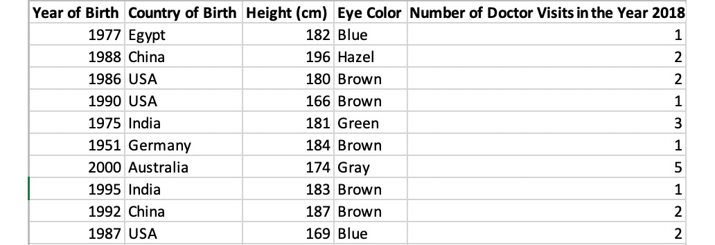
Figure 1.2: Healthcare data
When given a dataset, it's often helpful to classify the underlying data. In this case, the unit of observation for the dataset is an individual patient, because each row represents an individual observation, which is a unique patient. There are 10 data points, each with 5 variables. Three of the columns, Year of Birth, Height, and Number of Doctor Visits, are quantitative because they are represented by numbers. Two of the columns, Eye Color and Country of Birth, are qualitative.
Activity 1: Classifying a New Dataset
In this activity, we will classify the data in a dataset. You are about to start a job in a new city at an up-and-coming start-up. You're excited to start your new job, but you've decided to sell all your belongings before you head off. This includes your car. You're not sure at what price to sell it for, so you decide to collect some data. You ask some friends and family who recently sold their cars what the make of the car was, and how much they sold the cars for. Based on this information, you now have a dataset.
The data is as follows:
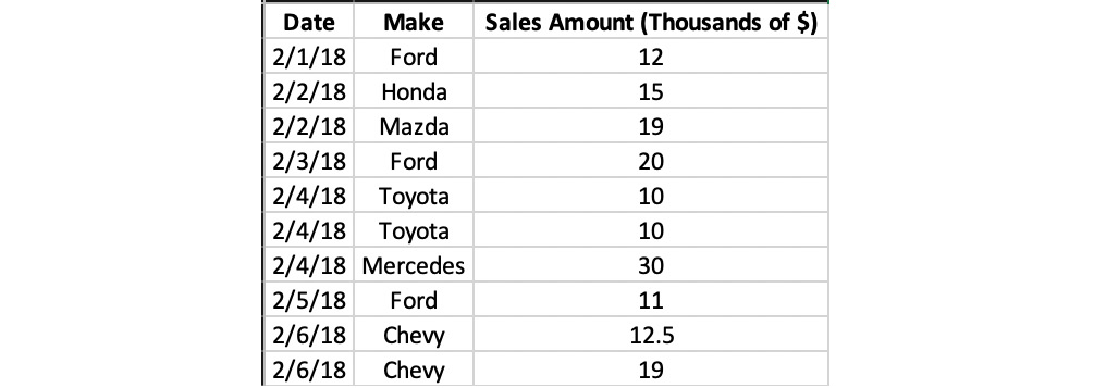
Figure 1.3: Used car sales data
Steps to follow:
- Determine the unit of observation.
- Classify the three columns as either quantitative or qualitative.
- Convert the Make column into quantitative data columns.
Note
The solution for this activity can be found via this link.