Consider an example of the real-world supervised ML algorithm called linear regression. In general, linear regression is an approach for modeling a target value (dependent value) based on an explanatory value (independent value). This method is used for forecasting and finding relationships between values. We can classify regression methods by the number of inputs (independent variables) and the type of relationship between the inputs and outputs (dependent variables).

Simple linear regression is the case where the number of independent variables is 1, and there is a linear relationship between the independent (x) and dependent (y) variable.

Linear regression is widely used in different areas, such as scientific research, where it can describe relationships between variables, as well as in applications within industry, such as a revenue prediction. For example, it can estimate a trend line that represents the long-term movement in the stock price time-series data. It tells whether the interest value of in a specific dataset has increased or decreased over the given period, as illustrated in the following screenshot:

If we have one input variable (independent variable) and one output variable (dependent variable) the regression is called simple, and we use the term simple linear regression for it. With multiple independent variables, we call this multiple linear regression or multivariable linear regression. Usually, when we are dealing with real-world problems, we have a lot of independent variables, so we model such problems with multiple regression models. Multiple regression models have a universal definition that covers other types, so even simple linear regression is often defined using the multiple regression definition.

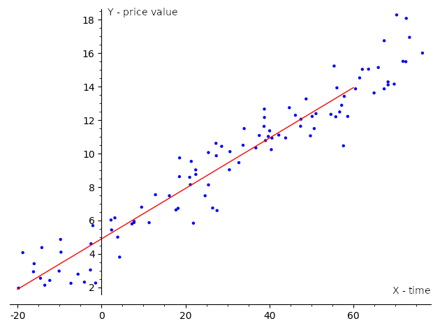
Assume that we have a dataset, , so that we can express the linear relation between y and x with mathematical formula in the following way:

Here, p is the dimension of the independent variable, and T denotes the transpose, so that is the inner product between vectors and β. Also, we can rewrite the previous expression in matrix notation, as follows:

,,,

The preceding matrix notation can be explained as follows:

• y: This is a vector of observed target values.
• x: This is a matrix of row-vectors, , which are known as explanatory or independent values.
• ß: This is a (p+1) dimensional parameters vector.
• ε: This is called an error term or noise. This variable captures all other factors that influence the y dependent variable other than the regressors.

When we are considering simple linear regression, p is equal to 1, and the equation will look like this:

The goal of the linear regression task is to find parameter vectors that satisfy the previous equation. Usually, there is no exact solution to such a system of linear equations, so the task is to estimate parameters that satisfy these equations with some assumptions. One of the most popular estimation approaches is one based on the principle of least squares: minimizing the sum of the squares of the differences between the observed dependent variable in the given dataset and those predicted by the linear function. This is called the ordinary least squares (OLS) estimator. So, the task can be formulated with the following formula:

In the preceding formula, the objective function S is given by the following matrix notation:

This minimization problem has a unique solution, in the case that the p columns of the x matrix are linearly independent. We can get this solution by solving the normal equation, as follows:

Linear algebra libraries can solve such equations directly with an analytical approach, but it has one significant disadvantage—computational cost. In the case of large dimensions of y and x, requirements for computer memory amount and computational time are too big to solve real-world tasks.

So, usually, this minimization task is solved with iterative approaches. Gradient descent (GD) is an example of such an algorithm. GD is a technique based on the observation that if the function is defined and is differentiable in a neighborhood of a point , then decreases fastest when it goes in the direction of the negative gradient of S at the point .

We can change our objective function to a form more suitable for an iterative approach. We can use the mean squared error (MSE) function, which measures the difference between the estimator and the estimated value, as illustrated here:

In the case of the multiple regression, we take partial derivatives for this function for each of x components, as follows:

So, in the case of the linear regression, we take the following derivatives:

The whole algorithm has the following description:

1. Initialize β with zeros.
2. Define a value for the learning rate parameter that controls how much we are adjusting parameters during the learning procedure.
3. Calculate the following values of β:

4. Repeat steps 1-3 for a number of times or until the MSE value reaches a reasonable amount.

The previously described algorithm is one of the simplest supervised ML algorithms. We described it with the linear algebra concepts we introduced earlier in the chapter. Later, it became more evident that almost all ML algorithms use linear algebra under the hood. The following samples show the higher-level API in different linear algebra libraries for solving the linear regression task, and we provide them to show how libraries can simplify the complicated math used underneath. We will give the details of the APIs used in these samples in the following chapters.

There are several iterative methods for solving problems of the form in the Eigen library. The LeastSquaresConjugateGradient class is one of them, which allows us to solve linear regression problems with the conjugate gradient algorithm. The ConjugateGradient algorithm can converge more quickly to the function's minimum than regular GD but requires that matrix A is positively defined to guarantee numerical stability. The LeastSquaresConjugateGradient class has two main settings: the maximum number of iterations and a tolerance threshold value that is used as a stopping criteria as an upper bound to the relative residual error, as illustrated in the following code block:

typedef float DType;
using Matrix = Eigen::Matrix<DType, Eigen::Dynamic, Eigen::Dynamic>;
int n = 10000;
Matrix x(n,1);
Matrix y(n,1);
Eigen::LeastSquaresConjugateGradient<Matrix> gd;
gd.setMaxIterations(1000);
gd.setTolerance(0.001) ;
gd.compute(x);
auto b = dg.solve(y);

For new x inputs, we can predict new y values with matrices operations, as follows:

Eigen::Matrixxf new_x(5, 2);
new_x << 1, 1, 1, 2, 1, 3, 1, 4, 1, 5;
auto new_y = new_x.array().rowwise() * b.transpose().array();

Also, we can calculate parameter's b vector (the linear regression task solution) by solving the normal equation directly, as follows:

auto b = (x.transpose() * x).ldlt().solve(x.transpose() * y);

Shogun is an open source ML library that provides a wide range of unified ML algorithms. The Shogun library has the CLinearRidgeRegression class for solving simple linear regression problems. This class solves problems with standard Cholesky matrix decomposition in a noniterative way, as illustrated in the following code block:

auto x = some<CDenseFeatures<float64_t>>(x_values);
auto y= some<CRegressionLabels>(y_values); // real-valued labels
float64_t tau_regularization = 0.0001;
auto lr = some<CLinearRidgeRegression>(tau_regularization, nullptr, nullptr); // regression model with regularization
lr->set_labels(y);
r->train(x)

For new x inputs, we can predict new y values in the following way:

auto new_x = some<CDenseFeatures<float64_t>>(new_x_values);
auto y_predict = lr->apply_regression(new_x);

Also, we can get the calculated parameters (the linear regression task solution) vector, as follows:

auto weights = lr->get_w();

Moreover, we can calculate the value of MSE, as follows:

auto y_predict = lr->apply_regression(x);
auto eval = some<CMeanSquaredError>();
auto mse = eval->evaluate(y_predict , y);

The Shark-ML library provides the LinearModel class for representing linear regression problems. There are two trainer classes for this kind of model: the LinearRegression class, which provides analytical solutions, and the LinearSAGTrainer class, which provides a stochastic average gradient iterative method, as illustrated in the following code block:

using namespace shark;
using namespace std;
Data<RealVector> x;
Data<RealVector> y;
RegressionDataset data(x, y);
LinearModel<> model;

LinearRegression trainer;
trainer.train(model, data);

We can get the calculated parameters (the linear regression task solution) vector by running the following code:

auto b = model.parameterVector();

For new x inputs, we can predict new y values in the following way:

Data<RealVector> new_x;
Data<RealVector> prediction = model(new_x);

Also, we can calculate the value of squared error, as follows:

SquaredLoss<> loss;
auto se = loss(y, prediction)

The Dlib library provides the krr_trainer class, which can get the template argument of the linear_kernel type to solve linear regression tasks. This class implements direct analytical solving for this type of problem with the kernel ridge regression algorithm, as illustrated in the following code block:

std::vector<matrix<double>> x;
std::vector<float> y;
krr_trainer<KernelType> trainer;
trainer.set_kernel(KernelType());
decision_function<KernelType> df = trainer.train(x, y);

For new x inputs, we can predict new y values in the following way:

std::vector<matrix<double>> new_x;
for (auto& v : x) {
    auto prediction = df(v);
    std::cout << prediction << std::endl;
}