

Jupyter Features
Having familiarized ourselves with the interface of two platforms for running Notebooks (Jupyter Notebook and JupyterLab), we are ready to start writing and running some more interesting examples.
Note
For the remainder of this book, you are welcome to use either the Jupyter Notebook platform or JupyterLab to follow along with the exercises and activities. The experience is similar, and you will be able to follow along seamlessly either way. Most of the screenshots for the remainder of this book have been taken from JupyterLab.
Jupyter has many appealing core features that make for efficient Python programming. These include an assortment of things, such as tab completion and viewing docstrings—both of which are very handy when writing code in Jupyter. We will explore these and more in the following exercise.
Note
The official IPython documentation can be found here: https://ipython.readthedocs.io/en/stable/. It provides details of the features we will discuss here, as well as others.
Exercise 1.03: Demonstrating the Core Jupyter Features
In this exercise, we'll relaunch the Jupyter platform and walk through a Notebook to learn about some core features, such as navigating workbooks with keyboard shortcuts and using magic functions. Follow these steps to complete this exercise:
- Start up one of the following platforms for running Jupyter Notebooks:
JupyterLab (run
jupyter lab)Jupyter Notebook (run
jupyter notebook)Then, open the platform in your web browser by copying and pasting the URL, as prompted in the Terminal.
Note
Here's the list of basic keyboard shortcuts; these are especially helpful if you wish to avoid having to use the mouse so often, which will greatly speed up your workflow.
Shift + Enter to run a cell
Esc to leave a cell
a to add a cell above
b to add a cell below
dd to delete a cell
m to change a cell to Markdown (after pressing Esc)
y to change a cell to code (after pressing Esc)
Arrow keys to move cells (after pressing Esc)
Enter to enter a cell
You can get help by adding a question mark to the end of any object and running the cell. Jupyter finds the docstring for that object and returns it in a pop-up window at the bottom of the app.
- Import
numpyand get thearrangedocstring, as follows:import numpy as np np.arange?
The output will be similar to the following:

Figure 1.28: The docstring for np.arange
- Get the Python
sortedfunction docstring as follows:sorted?
The output is as follows:

Figure 1.29: The docstring for sort
- You can pull up a list of the available functions on an object. You can do this for a NumPy array by running the following command:
a = np.array([1, 2, 3])
a.*?
Here's the output showing the list:

Figure 1.30: The output after running a.*?
- Click an empty code cell in the
Tab Completionsection. Typeimport(including the space after) and then press the Tab key:import <tab>
Tab completion can be used to do the following:
- List the available modules when importing external libraries:
from numpy import <tab>
- List the available modules of imported external libraries:
np.<tab>
- Perform function and variable completion:
np.ar<tab>
sor<tab>([2, 3, 1])
myvar_1 = 5
myvar_2 = 6
my<tab>
Test each of these examples for yourself in the following cells:

Figure 1.31: An example of tab completion for variable names
Note
Tab completion is different in the JupyterLab and Jupyter Notebook platforms. The same commands may not work on both.
Tab completion can be especially useful when you need to know the available input arguments for a module, explore a new library, discover new modules, or simply speed up the workflow. They will save time writing out variable names or functions and reduce bugs from typos. Tab completion works so well that you may have difficulty coding Python in other editors after today.
- List the available magic commands, as follows:
%lsmagic
The output is as follows:

Figure 1.32: Jupyter magic functions
Note
If you're running JupyterLab, you will not see the preceding output. A list of magic functions, along with information about each, can be found here: https://ipython.readthedocs.io/en/stable/interactive/magics.html.
The percent signs,
%and%%, are one of the basic features of Jupyter Notebook and are called magic commands. Magic commands starting with%%will apply to the entire cell, while magic commands starting with%will only apply to that line. - One example of a magic command that you will see regularly is as follows. This is used to display plots inline, which avoids you having to type
plt.show()each time you plot something. You only need to execute it once at the beginning of the session:%matplotlib inline
The timing functions are also very handy magic functions and come in two varieties: a standard timer
(%timeor%%time) and a timer that measures the average runtime of many iterations (%timeitand%%timeit). We'll see them being used here. - Declare the
avariable, as follows:a = [1, 2, 3, 4, 5] * int(1e5)
- Get the runtime for the entire cell, as follows:
%%time
for i in range(len(a)):
    a[i] += 5
The output is as follows:
CPU times: user 68.8 ms, sys: 2.04 ms, total: 70.8 ms
Wall time: 69.6 ms
- Get the runtime for one line:
%time a = [_a + 5 for _a in a]
The output is as follows:
CPU times: user 21.1 ms, sys: 2.6 ms, total: 23.7 ms
Wall time: 23.1 ms
- Check the average results of multiple runs, as follows:
%timeit set(a)
The output is as follows:
4.72 ms ± 55.5 µs per loop (mean ± std. dev. of 7 runs, 100 loops each)
Note the difference in use between one and two percent signs. Even when using a Python kernel (as you are currently doing), other languages can be invoked using magic commands. The built-in options include JavaScript, R, Perl, Ruby, and Bash. Bash is particularly useful as you can use Unix commands to find out where you are currently (
pwd), see what's in the directory (ls), make new folders (mkdir), and write file contents (cat/head/tail).Note
Notice how list comprehensions are quicker than loops in Python. This can be seen by comparing the wall time for the first and second cell, where the same calculation is done significantly faster with list comprehension. Please note that the step 15-18 are Linux-based commands. If you are working on other operating systems like Windows and MacOS, these steps might not work.
- Write some text into a file in the working directory, print the directory's contents, print an empty line, and then write back the contents of the newly created file before removing it, as follows:
%%bash
echo "using bash from inside Jupyter!" > test-file.txt
ls
echo ""
cat test-file.txt
rm test-file.txt
The output is as follows:

Figure 1.33: Running a bash command in Jupyter
- List the contents of the working directory with
ls, as follows:%ls
The output is as follows:
chapter_1_workbook.ipynb
- List the path of the current working directory with
pwd. Notice how we needed to use the%%bashmagic function forpwd, but not forls:%%bash pwd
The output is as follows:
/Users/alex/Documents/The-Applied-Data-Science-Workshop/chapter-01
- There are plenty of external magic commands that can be installed. A popular one is
ipython-sql, which allows for SQL code to be executed in cells.Jupyter magic functions can be installed the same way as PyPI Python libraries, using
piporconda. Open a new Terminal window and execute the following code to installipython-sql:pip install ipython-sql
- Run the
%load_ext sqlcell to load the external command into the Notebook.This allows connections to be made to remote databases so that queries can be executed (and thereby documented) right inside the Notebook.
- Now, run the sample SQL query, as follows:
%%sql sqlite://
SELECT *
FROM (
    SELECT 'Hello' as msg1, 'World!' as msg2
);
The output is as follows:

Figure 1.34: Running a SQL query in Jupyter
Here, we connected to the local
sqlitesource withsqlite://; however, this line could instead point to a specific database on a local or remote server. For example, a.sqlitedatabase file on your desktop could be connected to with the line%sql sqlite:////Users/alex/Desktop/db.sqlite, where the username in this case isalexand the file isdb.sqlite.After connecting, we execute a simple
SELECTcommand to show how the cell has been converted to run SQL code instead of Python. - Earlier in this chapter, we went over the instructions for installing the
watermarkexternal library, which helps to document versioning in the Notebook. If you haven't installed it yet, then open a new window and run the following code:pip install watermark
Once installed, it can be imported into any Notebook using
%load_ext watermark. Then, it can be used to document library versions and system hardware. - Load and call the
watermarkmagic function and call its docstring with the following command:%load_ext watermark %watermark?
The output is as follows:

Figure 1.35: The docstring for watermark
Notice the various arguments that can be passed in when calling it, such as
-afor author,-vfor the Python version,-mfor machine information, and-dfor date. - Use the
watermarklibrary to add version information to the notebook, as follows:Note
The code snippet shown here uses a backslash (
\) to split the logic across multiple lines. When the code is executed, Python will ignore the backslash, and treat the code on the next line as a direct continuation of the current line.%watermark -d -v -m -p \ requests,numpy,pandas,matplotlib,seaborn,sklearn
The output is as follows:

Figure 1.36: watermark output in the Notebook
Note
To access the source code for this specific section, please refer to https://packt.live/30KoAfu.
You can also run this example online at https://packt.live/2Y49zTQ.
In this exercise, we looked at the core features of Jupyter, including tab completion and magic functions. You'll review these features and have a chance to test them out yourself in the activity at the end of this chapter.
Converting a Jupyter Notebook into a Python Script
In this section, we'll learn how to convert a Jupyter Notebook into a Python script. This is equivalent to copying and pasting the contents of each code cell into a single .py file. The Markdown sections are also included as comments.
It can be beneficial to convert a Notebook into a .py file because the code is then available in plain text format. This can be helpful for version control— to see the difference in code between two versions of a Notebook, for example. It can also be a helpful trick for extracting chunks of code.
This conversion can be done from the Jupyter Dashboard (File -> Download as) or by opening a new Terminal window, navigating to the chapter-02 folder, and executing the following:
jupyter nbconvert --to=python chapter_2_workbook.ipynb
The output is as follows:
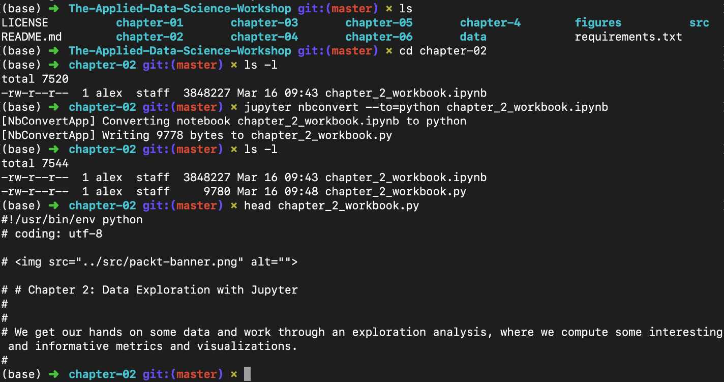
Figure 1.37: Converting a Notebook into a script (.py) file
Note that we are using the next chapter's Notebook for this example.
Another benefit of converting Notebooks into .py files is that, when you want to determine the Python library requirements for a Notebook, the pipreqs tool will do this for us, and export them into a requirements.txt file. This tool can be installed by running the following command:
pip install pipreqs
You might require root privileges for this.
This command is called from outside the folder containing your .py files. For example, if the .py files are inside a folder called chapter-02, you could do the following:
pipreqs chapter-02/
The output is as follows:
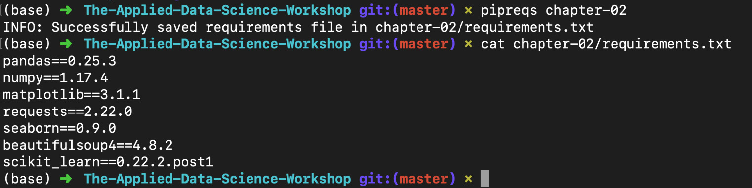
Figure 1.38: Using pipreqs to generate a requirements.txt file
The resulting requirements.txt file for chapter_2_workbook.ipynb will look similar to the following:
cat chapter-02/requirements.txt
matplotlib==3.1.1
seaborn==0.9.0
numpy==1.17.4
pandas==0.25.3
requests==2.22.0
beautifulsoup4==4.8.1
scikit_learn==0.22
Python Libraries
Having now seen all the basics of Jupyter Notebooks, and even some more advanced features, we'll shift our attention to the Python libraries we'll be using in this book.
Libraries, in general, extend the default set of Python functions. Some examples of commonly used standard libraries are datetime, time, os, and sys. These are called standard libraries because they are included with every installation of Python.
For data science with Python, the most heavily relied upon libraries are external, which means they do not come as standard with Python.
The external data science libraries we'll be using in this book are numpy, pandas, seaborn, matplotlib, scikit-learn, requests, and bokeh.
Note
It's a good idea to import libraries using industry standards—for example, import numpy as np. This way, your code is more readable. Try to avoid doing things such as from numpy import *, as you may unwittingly overwrite functions. Furthermore, it's often nice to have modules linked to the library via a dot (.) for code readability.
Let's briefly introduce each:
numpyoffers multi-dimensional data structures (arrays) that operations can be performed on. This is far quicker than standard Python data structures (such as lists). This is done in part by performing operations in the background using C. NumPy also offers various mathematical and data manipulation functions.pandasis Python's answer to the R DataFrame. It stores data in 2D tabular structures where columns represent different variables and rows correspond to samples. pandas provides many handy tools for data wrangling, such as filling inNaNentries and computing statistical descriptions of the data. Working with pandas DataFrames will be a big focus of this book.matplotlibis a plotting tool inspired by the MATLAB platform. Those familiar with R can think of it as Python's version ofggplot. It's the most popular Python library for plotting figures and allows for a high level of customization.seabornworks as an extension ofmatplotlib, where various plotting tools that are useful for data science are included. Generally speaking, this allows for analysis to be done much faster than if you were to create the same things manually with libraries such asmatplotlibandscikit-learn.scikit-learnis the most commonly used machine learning library. It offers top-of-the-line algorithms and a very elegant API where models are instantiated and then fit with data. It also provides data processing modules and other tools that are useful for predictive analytics.requestsis the go-to library for making HTTP requests. It makes it straightforward to get HTML from web pages and interface with APIs. For parsing HTML, many chooseBeautifulSoup4, which we'll cover in Chapter 6, Web Scraping with Jupyter Notebooks.
We'll start using these libraries in the next chapter.
Activity 1.01: Using Jupyter to Learn about pandas DataFrames
We are going to be using pandas heavily in this book. In particular, any data that's loaded into our Notebooks will be done using pandas. The data will be contained in a DataFrame object, which can then be transformed and saved back to disk afterward. These DataFrames offer convenient methods for running calculations over the data for exploration, visualization, and modeling.
In this activity, you'll have the opportunity to use pandas DataFrames, along with the Jupyter features that have been discussed in this section. Follow these steps to complete this activity:
- Start up one of the platforms for running Jupyter Notebooks and open it in your web browser by copying and pasting the URL, as prompted in the Terminal.
Note
While completing this activity, you will need to use many cells in the Notebook. Please insert new cells as required.
- Import the pandas and NumPy libraries and assign them to the
pdandnpvariables, respectively. - Pull up the docstring for
pd.DataFrame. Scan through the Parameters section and read the Examples section. - Create a dictionary with
fruitandscorekeys, which correspond to list values with at least three items in each. Ensure that you give your dictionary a suitable name (note that in Python, a dictionary is a collection of values); for example,{"fruit": ["apple", ...], "score": [8, ...]}. - Use this dictionary to create a DataFrame. You can do this using
pd.DataFrame(data=name of dictionary). Assign it to thedfvariable. - Display this DataFrame in the Notebook.
- Use tab completion to pull up a list of functions available for
df. - Pull up the docstring for the
sort_valuesDataFrame function and read through the Examples section. - Sort the DataFrame by score in descending order. Try to see how many times you can use tab completion as you write the code.
- Use the
timeitmagic function to test how long this sorting operation takes.Note
The detailed steps for this activity, along with the solutions, can be found via this link