

What data modeling means in Power BI
Data modeling is undoubtedly one of the most important parts of Power BI development. The purpose of data modeling in Power BI is different from data models in transactional systems. In a transactional system, the goal is to have a model that is optimized for recording transactional data. Nevertheless, a well-designed data model in Power BI must be optimized for querying the data and reducing the dataset size by aggregating that data.
While not everyone has the luxury of having a prebuilt data warehouse, you end up creating a data model in Power BI in many cases. It is very tempting to get the whole data as is from various data sources and import it to Power BI. Answering business questions can quickly translate to complex queries that take a long time to process, which is not ideal. So, it is highly advised to resist the temptation to import everything from the data sources into Power BI and solve the problems later. Instead, it is wise to try to get your data model right so that it is capable of precisely answering business-driven questions in the most performant way. When modeling data in Power BI, you need to build a data model based on the business logic. Having said that, you may need to join different tables and aggregate your data to a certain level that answers all business-driven questions. It can get worse if you have data from various data sources of different grains representing the same logic.
Therefore, you need to transform and reshape that data before loading it to the data model in Power BI. Power Query is the right tool to take care of all that. After we cut all the noise from our data, we have a clean, easy-to-understand, and easy-to-work-with data model.
Semantic model
Power BI inherits its blood from Power Pivot and SSAS Tabular models. All of them use the xVelocity engine, an updated version of the VertiPaq engine designed for in-memory data analysis and consisting of semantic model objects such as tables, relationships, hierarchies, and measures, which are stored in memory, leveraging column store indexing. All of this means that you would expect to get tremendous performance gains over highly compressed data, right? Well, it depends. If you efficiently transformed the data to support business logic, then you can expect to have fast and responsive reports. After you import your data into the data model in Power BI, you have built a semantic model when it comes to the concepts. A semantic model is a unified data model that provides business contexts to data. The semantic model can be accessed from various tools to visualize data without needing it to be transformed again. In that sense, when you publish your reports to the Power BI service, you can analyze the dataset in Excel or use third-party tools such as Tableau to connect to a Power BI dataset backed by a Premium capacity and visualize your data.
Building an efficient data model in Power BI
An efficient data model can quickly answer all business questions that you are supposed to answer; it is easy to understand and easy to maintain. Let's analyze the preceding sentence. Your model must do the following:
- Perform well (quickly)
- Be business-driven
- Decrease the level of complexity (be easy to understand)
- Be maintainable with low costs
Let's look at the preceding points with a scenario.
You are tasked to create a report on top of three separate data sources, as follows:
- An OData data source with 15 tables. The tables have between 50 and 250 columns.
- An Excel file with 20 sheets that are interdependent with many formulas.
- A data warehouse hosted in SQL Server. You need to get data from five dimensions and two fact tables:
- Of those five dimensions, one is a Date dimension and the other is a Time dimension. The grain of the Time dimension is hour, minute.
- Each of the fact tables has between 50 and 200 million rows. The grain of both fact tables from a date and time perspective is day, hour, minute.
- Your organization has a Power BI Pro license.
There are already a lot of important points in the preceding scenario that you must consider before starting to get the data from the data sources. There are also a lot of points that are not clear at this stage. I have pointed out some of them:
- OData: OData is an online data source, so it could be slow to load the data from the source system.
The tables are very wide so it can potentially impact the performance.
Our organization has a Power BI Pro license, so we are limited to 1 GB file size.
The following questions should be answered by the business. Without knowing the answers, we may end up building a report that is unnecessarily large with poor performance. This can potentially lead to the customer's dissatisfaction:
(a) Do we really need to import all the columns from those 15 tables?
(b) Do we also need to import all data or is just a portion of the data enough? In other words, if there is 10-years worth of data kept in the source system, does the business need to analyze all the data, or does just 1 or 2 years of data fit the purpose?
- Excel: Generally, Excel workbooks with many formulas can be quite hard to maintain. So, we need to ask the following questions of the business:
(a) How many of those 20 sheets of data are going to be needed by the business? You may be able to exclude some of those sheets.
(b) How often are the formulas in the Excel file edited? This is a critical point as modifying the formulas can easily break your data processing in Power Query and generate errors. So, you would need to be prepared to replicate a lot of formulas in Power BI if needed.
- Data warehouse in SQL Server: It is beneficial to have a data warehouse as a source system as data warehouses normally have a much better structure from an analytical viewpoint. But in our scenario, the finest grain of both fact tables is down to a minute. This can potentially turn into an issue pretty quickly. Remember, we have a Power BI Pro license, so we are limited to a 1 GB file size only. Therefore, it is wise to clarify some questions with the business before we start building the model:
(a) Does the business need to analyze all the metrics down to the minute or is day-level enough?
(b) Do we need to load all the data into Power BI, or is a portion of the data enough?
We now know the questions to ask, but what if the business needs to analyze the whole history of the data? In that case, we may consider using composite models with aggregations.
Having said all that, there is another point to consider. We already have five dimensions in the data warehouse. Those dimensions can potentially be reused in our data model. So, it is wise to look at the other data sources and find commonalities in the data patterns.
You may come up with some more legitimate points and questions. However, you can quickly see in the previously mentioned points and questions that you need to talk to the business and ask questions before starting the job. It is a big mistake to start getting data from the source systems before framing your questions around business processes, requirements, and technology limitations. There are also some other points that you need to think about from a project management perspective that are beyond the scope of this book.
The initial points to take into account for building an efficient data model are as follows:
- We need to ask questions of the business to avoid any confusions and potential reworks in the future.
- We need to understand the technology limitations and come up with solutions.
- We have to have a good understanding of data modeling, so we can look for common data patterns to prevent overlaps.
At this point, you may think, "OK, but how we can get there?" My answer is that you have already taken the first step, which is reading this book. All the preceding points and more are covered in this book. The rest is all about you and how you apply your learning to your day-to-day challenges.
Star schema (dimensional modeling) and snowflaking
First things first, star schema and dimensional modeling are the same things. In Power BI data modeling, the term star schema is more commonly used. So, in this book, we will use the term star schema. The intention of this book is not to teach you about dimensional modeling. Nevertheless, we'll focus on how to model data using star schema data modeling techniques. We will remind you of some star schema concepts.
Transactional modeling versus star schema modeling
In transactional systems, the main goal is to improve the system's performance in creating new records and updating/deleting existing records. So, it is essential to go through the normalization process to decrease data redundancy and increase data entry performance when designing transactional systems. In a straightforward form of normalization, we break tables down into master-detail tables.
But the goal of a business analysis system is very different. In business analysis, we need a data model optimized for querying in the most performant way.
Let's continue with a scenario.
Say we have a transactional retail system for international retail stores. We have hundreds of transactions every second from different parts of the world. The company owner wants to see the total sales amount in the past 6 months.
This calculation sounds easy. It is just a simple SUM of sales. But wait, we have hundreds of transactions every second, right? If we have only 100 transactions per second, then we have 8,640,000 transactions a day. So, for 6 months of data, we have more than 1.5 billion rows. Therefore, a simple SUM of sales will take a reasonable amount of time to process.
The scenario continues: Now, a new query comes from the business. The company owner now wants to see the total sales amount in the past 6 months by country and city. He simply wants to know what the best-selling cities are.
We need to add another condition to our simple SUM calculation, which translates to a join to the geography table. For those coming from a relational database design background, it will be obvious that joins are relatively expensive operations. This scenario can go on and on. So, you can imagine how quickly you will face a severe issue.
In the star schema, however, we already joined all those tables based on business entities. We aggregated and loaded the data into denormalized tables. In the preceding scenario, the business is not interested in seeing every transaction at the second level. We can summarize the data at the day level, which decreases the number of rows from 1.5 billion to a couple of thousands of rows for the whole 6 months. Now you can imagine how fast the summation would be running over thousands of rows instead of 1.5 billion rows.
The idea of the star schema is to keep all numeric values in separate tables called fact tables and put all descriptive information into other tables called dimension tables. Usually, the fact tables are surrounded by dimensions that explain those facts. When you look at a data model with a fact table in the middle surrounded by dimensions, you see that it looks like a star. Therefore, it is called a star schema. In this book, we generally use the Adventure Works DW data, a renowned Microsoft sample dataset, unless stated otherwise. Adventure Works is an international bike shop that sells products both online and in their retail shops. The following figure shows Internet Sales in a star schema shape:
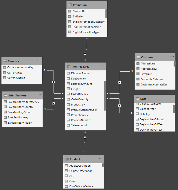
Figure 1.9 – Adventure Works DW, Internet Sales star schema
Snowflaking
Snowflaking is when you do not have a perfect star schema when dimension tables surround your fact tables. In some cases, you have some levels of descriptions stored in different tables. Therefore, some dimensions of your model are linked to some other tables that describe the dimensions in a greater level of detail. Snowflaking is normalizing the dimension tables. In some cases, snowflaking is inevitable; nevertheless, the general rule of thumb in data modeling in Power BI (when following a star schema) is to avoid snowflaking as much as possible. The following figure shows snowflaking in Adventure Works Internet Sales:
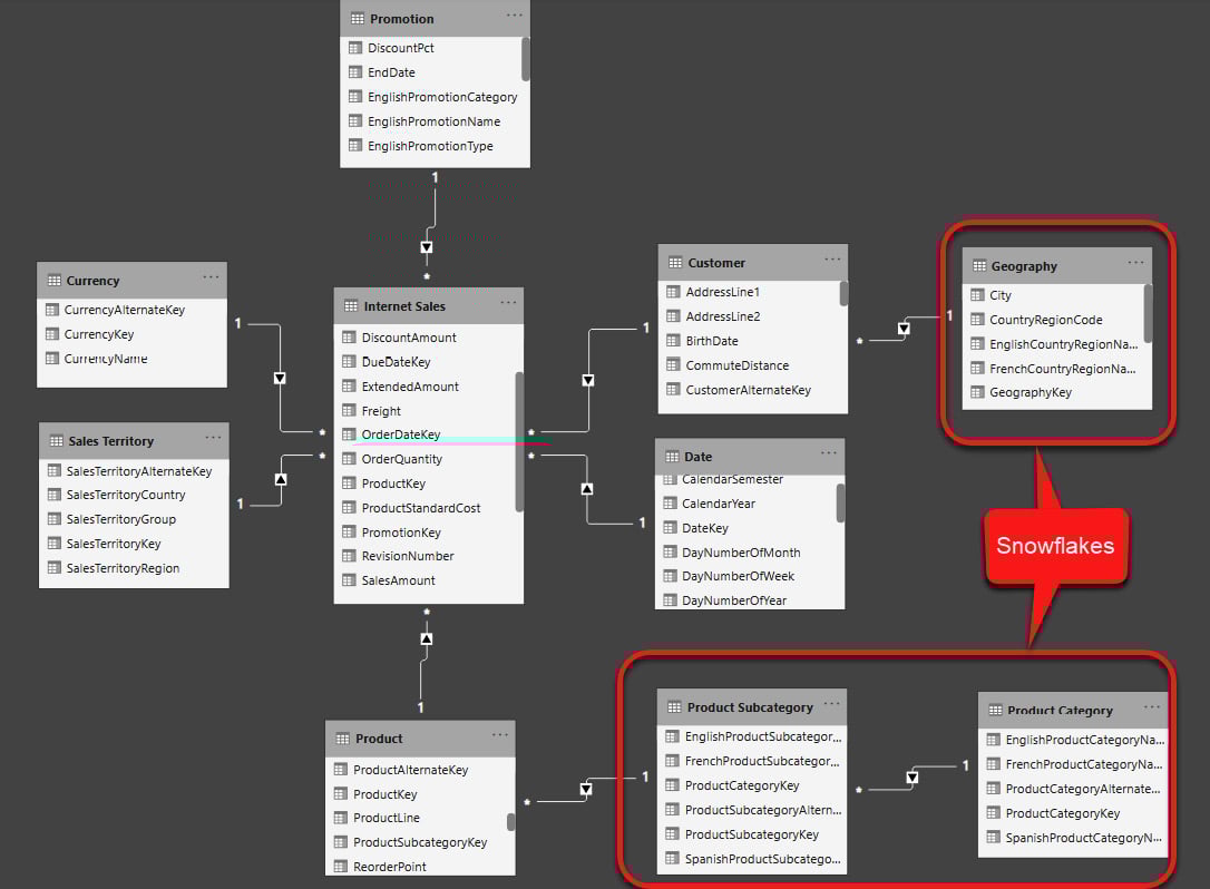
Figure 1.10 – Adventure Works, Internet Sales snowflakes
Understanding denormalization
In real-world scenarios, not everyone has the luxury of having a pre-built data warehouse designed in a star schema. In reality, snowflaking in data warehouse design is inevitable. So, you may build your data model on top of various data sources, including transactional database systems and non-transactional data sources such as Excel files and CSV files. So, you almost always need to denormalize your model to a certain degree. Depending on the business requirements, you may end up having some level of normalization along with some denormalization. The reality is that there is no specific rule for the level of normalization and denormalization. The general rule of thumb is to denormalize your model so that a dimension can describe all the details as much as possible.
In the preceding example from Adventure Works DW, we have snowflakes of Product Category and Product Subcategory that can be simply denormalized into the Product dimension.
Let's go through a hands-on exercise.
Go through the following steps to denormalize Product Category and Product Subcategory into the Product dimension.
Note
You can download the Adventure Works, Internet Sales.pbix file from here:
Open the Adventure Works, Internet Sales.pbix file and follow these steps:
- Click Transform data on the Home tab in the Queries section.
- Click the Product Query.
- Click Merge Queries on the Home tab in the Combine section.
- Select Product Subcategory from the drop-down list.
- Click ProductSubcategoryKey on the Product table.
- Click ProductSubcategoryKey on the Product Subcategory table.
- Select Left Outer (all from first matching from the second) from the Join Kind dropdown.
- Click OK:
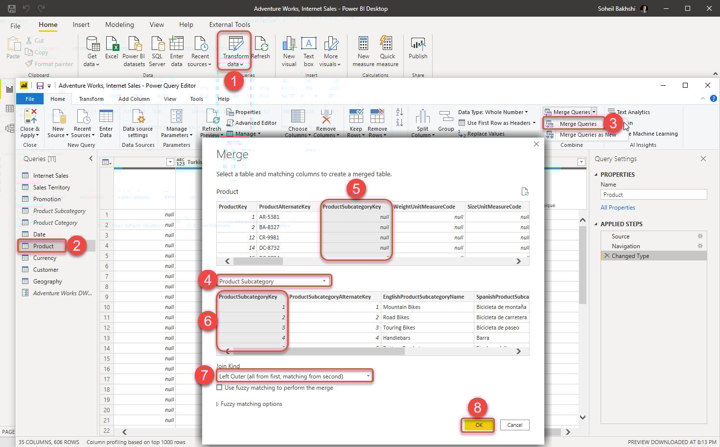
Figure 1.11 – Merging Product and Product Subcategory
This adds a new step named Merged Queries. As you see, the values of this column are all Table. This type of column is called Structured Column. The merging Product and Product Subcategory step creates a new structured column named Product Subcategory:
You will learn more about structured columns in Chapter 3, Data Preparation in Power Query Editor.
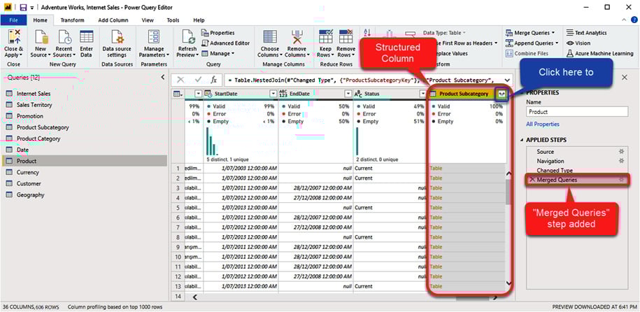
Figure 1.12 – Merging the Product and Product Subcategory tables
Now let's look at how to expand a structured column in the query editor:
- Click the Expand button to expand the Product Subcategory column.
- Select ProductCategoryKey.
- Select the EnglishProductSubcategoryName columns and unselect the rest.
- Unselect Use original column names as prefix.
- Click OK:
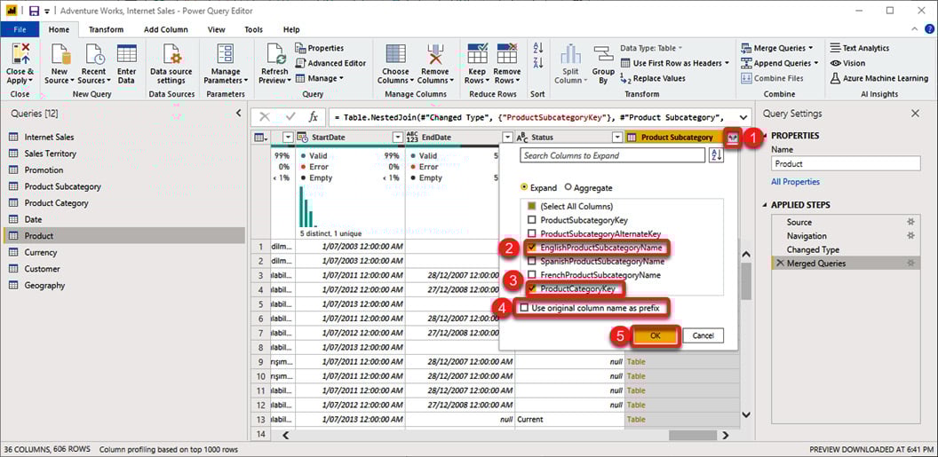
Figure 1.13 – Expanding Structured Column in the Query Editor
So far, we have added the EnglishProductSubcategoryName and ProductCategoryKey columns from the Product Subcategory query to the Product query. The next step is to add EnglishProductCategoryName from the Product Category query. To do so, we need to merge the Product query with Product Category:
- Click Merge Queries again.
- Select Product Category from the drop-down list.
- Select ProductCategoryKey from the Product table.
- Select ProductCategoryKey from the Product Category table.
- Select Left Outer (all from first matching from second).
- Click OK:
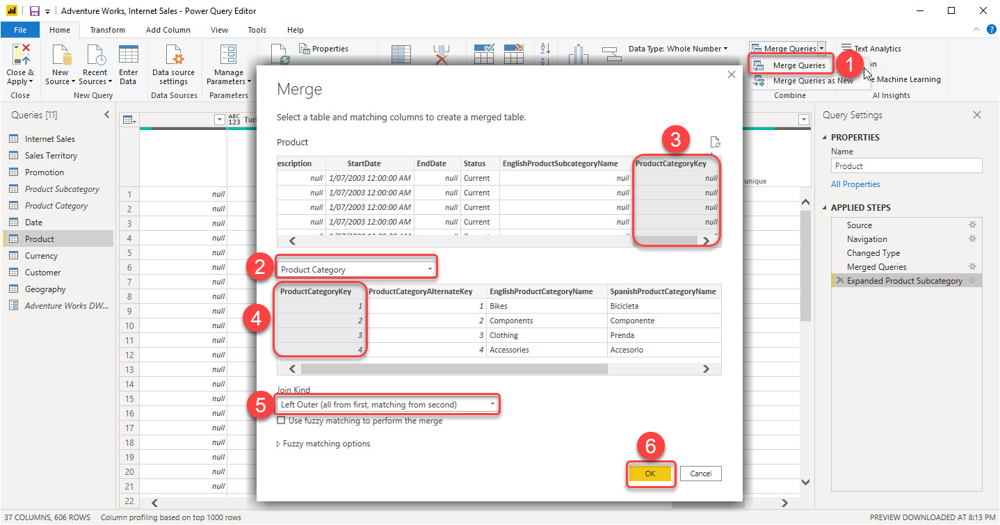
Figure 1.14 – Merging Product and Product Category
This adds another step and a new structured column named Product Category. We now need to do the following:
- Expand the new column.
- Pick EnglishProductCategoryName from the list.
- Unselect Use original column name as prefix.
- Click OK:
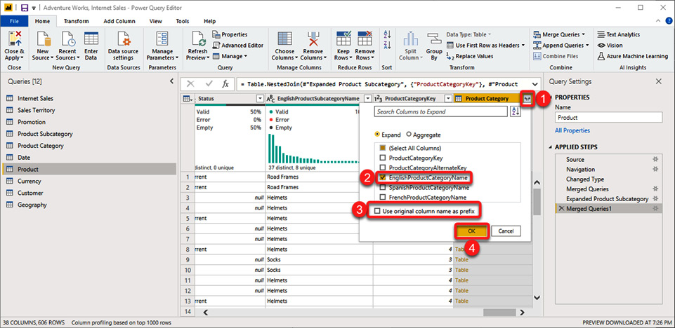
Figure 1.15 – Merging Product and Product Category
The next step is to remove the ProductCategoryKey column as we do not need it anymore. To do so, do the following:
- Click on the ProductCategoryKey column.
- Click the Remove Columns button in the Managed Column section of the Home tab:
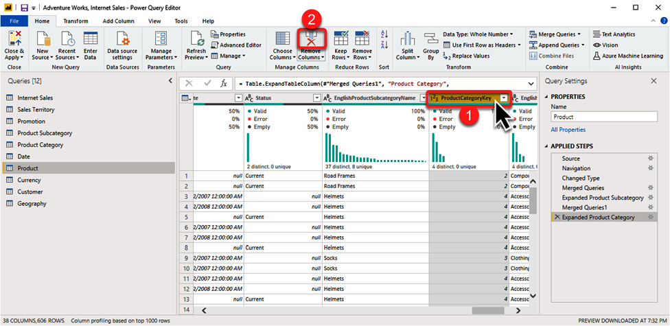
Figure 1.16 – Removing a column in the Query Editor
Now we have merged the Product Category and Product Subcategory snowflakes with the Product query. So, you have denormalized the snowflakes.
The very last step is to unload both the Product Category and Product Subcategory queries:
- Right-click on each query.
- Untick Enable load from the menu.
- Click Continue on the Possible Data Loss Warning pop-up message:
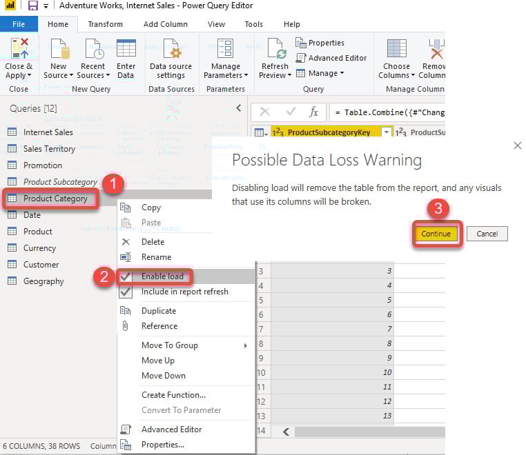
Figure 1.17 – Unloading queries in the Query Editor
Now we need to import the data into the data model by clicking Close & Apply:
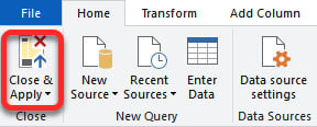
Figure 1.18 – Importing data into the data model
We have now achieved what we were after: we denormalized the Product Category and Product Subcategory tables, therefore rather than loading those two tables, we now have EnglishProductCategoryName and EnglishProductSubcategoryName represented as new columns in the Product table.
Job done!