

Introduction
The study and application of machine learning and artificial intelligence has recently been the source of much interest and research in the technology and business communities. Advanced data analytics and machine learning techniques have shown great promise in advancing many sectors, such as personalized healthcare and self-driving cars, as well as in solving some of the world's greatest challenges, such as combating climate change (see Tackling Climate Change with Machine Learning: https://arxiv.org/pdf/1906.05433.pdf).
This book has been designed to help you to take advantage of the unique confluence of events in the field of data science and machine learning today. Across the globe, private enterprises and governments are realizing the value and efficiency of data-driven products and services. At the same time, reduced hardware costs and open source software solutions are significantly reducing the barriers to entry of learning and applying machine learning techniques.
Here, we will focus on supervised machine learning (or, supervised learning for short). We'll explain the different types of machine learning shortly, but let's begin with some quick information. The now-classic example of supervised learning is developing an algorithm to distinguish between pictures of cats and dogs. The supervised part arises from two aspects; first, we have a set of pictures where we know the correct answers. We call such data labeled data. Second, we carry out a process where we iteratively test our algorithm's ability to predict "cat" or "dog" given pictures, and we make corrections to the algorithm when the predictions are incorrect. This process, at a high level, is similar to teaching children. However, it generally takes a lot more data to train an algorithm than to teach a child to recognize cats and dogs! Fortunately, there are rapidly growing sources of data at our disposal. Note the use of the words learning and train in the context of developing our algorithm. These might seem to be giving human qualities to our machines and computer programs, but they are already deeply ingrained in the machine learning (and artificial intelligence) literature, so let's use them and understand them. Training in our context here always refers to the process of providing labeled data to an algorithm and making adjustments to the algorithm to best predict the labels given the data. Supervised means that the labels for the data are provided within the training, allowing the model to learn from these labels.
Let's now understand the distinction between supervised learning and other forms of machine learning.
When to Use Supervised Learning
Generally, if you are trying to automate or replicate an existing process, the problem is a supervised learning problem. As an example, let's say you are the publisher of a magazine that reviews and ranks hairstyles from various time periods. Your readers frequently send you far more images of their favorite hairstyles for review than you can manually process. To save some time, you would like to automate the sorting of the hairstyle images you receive based on time periods, starting with hairstyles from the 1960s and 1980s, as you can see in the following figure:

Figure 1.1: Images of hairstyles from different time periods
To create your hairstyles-sorting algorithm, you start by collecting a large sample of hairstyle images and manually labeling each one with its corresponding time period. Such a dataset (known as a labeled dataset) is the input data (hairstyle images) for which the desired output information (time period) is known and recorded. This type of problem is a classic supervised learning problem; we are trying to develop an algorithm that takes a set of inputs and learns to return the answers that we have told it are correct.
Python Packages and Modules
Python is one of the most popular programming languages used for machine learning, and is the language used here.
While the standard features that are included in Python are certainly feature-rich, the true power of Python lies in the additional libraries (also known as packages), which, thanks to open source licensing, can be easily downloaded and installed through a few simple commands. In this book, we generally assume your system has been configured using Anaconda, which is an open source environment manager for Python. Depending on your system, you can configure multiple virtual environments using Anaconda, each one configured with specific packages and even different versions of Python. Using Anaconda takes care of many of the requirements to get ready to perform machine learning, as many of the most common packages come pre-built within Anaconda. Refer to the preface for Anaconda installation instructions.
In this book, we will be using the following additional Python packages:
- NumPy (pronounced Num Pie and available at https://www.numpy.org/): NumPy (short for numerical Python) is one of the core components of scientific computing in Python. NumPy provides the foundational data types from which a number of other data structures derive, including linear algebra, vectors and matrices, and key random number functionality.
- SciPy (pronounced Sigh Pie and available at https://www.scipy.org): SciPy, along with NumPy, is a core scientific computing package. SciPy provides a number of statistical tools, signal processing tools, and other functionality, such as Fourier transforms.
- pandas (available at https://pandas.pydata.org/): pandas is a high-performance library for loading, cleaning, analyzing, and manipulating data structures.
- Matplotlib (available at https://matplotlib.org/): Matplotlib is the foundational Python library for creating graphs and plots of datasets and is also the base package from which other Python plotting libraries derive. The Matplotlib API has been designed in alignment with the Matlab plotting library to facilitate an easy transition to Python.
- Seaborn (available at https://seaborn.pydata.org/): Seaborn is a plotting library built on top of Matplotlib, providing attractive color and line styles as well as a number of common plotting templates.
- Scikit-learn (available at https://scikit-learn.org/stable/): Scikit-learn is a Python machine learning library that provides a number of data mining, modeling, and analysis techniques in a simple API. Scikit-learn includes a number of machine learning algorithms out of the box, including classification, regression, and clustering techniques.
These packages form the foundation of a versatile machine learning development environment, with each package contributing a key set of functionalities. As discussed, by using Anaconda, you will already have all of the required packages installed and ready for use. If you require a package that is not included in the Anaconda installation, it can be installed by simply entering and executing the following code in a Jupyter notebook cell:
!conda install <package name>
As an example, if we wanted to install Seaborn, we'd run the following command:
!conda install seaborn
To use one of these packages in a notebook, all we need to do is import it:
import matplotlib
Loading Data in Pandas
pandas has the ability to read and write a number of different file formats and data structures, including CSV, JSON, and HDF5 files, as well as SQL and Python Pickle formats. The pandas input/output documentation can be found at https://pandas.pydata.org/pandas-docs/stable/user_guide/io.html. We will continue to look into the pandas functionality by loading data via a CSV file.
Note
The dataset used in this chapter is available on our GitHub repository via the following link: https://packt.live/2vjyPK9. Once you download the entire repository on your system, you can find the dataset in the Datasets folder. Furthermore, this dataset is the Titanic: Machine Learning from Disaster dataset, which was originally made available at https://www.kaggle.com/c/Titanic/data.
The dataset contains a roll of the guests on board the famous ship Titanic, as well as their age, survival status, and number of siblings/parents. Before we get started with loading the data into Python, it is critical that we spend some time looking over the information provided for the dataset so that we can have a thorough understanding of what it contains. Download the dataset and place it in the directory you're working in.
Looking at the description for the data, we can see that we have the following fields available:
survival: This tells us whether a given person survived (0= No,1= Yes).pclass: This is a proxy for socio-economic status, where first class is upper, second class is middle, and third class is lower status.sex: This tells us whether a given person is male or female.age: This is a fractional value if less than 1; for example, 0.25 is 3 months. If the age is estimated, it is in the form of xx.5.sibsp: A sibling is defined as a brother, sister, stepbrother, or stepsister, and a spouse is a husband or wife.parch: A parent is a mother or father, while a child is a daughter, son, stepdaughter, or stepson. Children that traveled only with a nanny did not travel with a parent. Thus, 0 was assigned for this field.ticket: This gives the person's ticket number.fare: This is the passenger's fare.cabin: This tells us the passenger's cabin number.embarked: The point of embarkation is the location where the passenger boarded the ship.
Note that the information provided with the dataset does not give any context as to how the data was collected. The survival, pclass, and embarked fields are known as categorical variables as they are assigned to one of a fixed number of labels or categories to indicate some other information. For example, in embarked, the C label indicates that the passenger boarded the ship at Cherbourg, and the value of 1 in survival indicates they survived the sinking.
Exercise 1.01: Loading and Summarizing the Titanic Dataset
In this exercise, we will read our Titanic dataset into Python and perform a few basic summary operations on it:
- Open a new Jupyter notebook.
- Import the
pandasandnumpypackages using shorthand notation:import pandas as pd import numpy as np
- Open the
titanic.csvfile by clicking on it in the Jupyter notebook home page as shown in the following figure: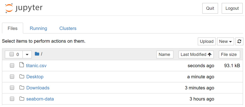
Figure 1.2: Opening the CSV file
The file is a CSV file, which can be thought of as a table, where each line is a row in the table and each comma separates columns in the table. Thankfully, we don't need to work with these tables in raw text form and can load them using
pandas: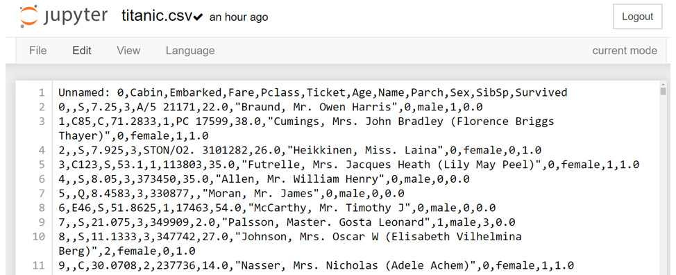
Figure 1.3: Contents of the CSV file
Note
Take a moment to look up the pandas documentation for the
read_csvfunction at https://pandas.pydata.org/pandas-docs/stable/reference/api/pandas.read_csv.html. Note the number of different options available for loading CSV data into a pandas DataFrame. - In an executable Jupyter notebook cell, execute the following code to load the data from the file:
df = pd.read_csv(r'..\Datasets\titanic.csv')
The pandas DataFrame class provides a comprehensive set of attributes and methods that can be executed on its own contents, ranging from sorting, filtering, and grouping methods to descriptive statistics, as well as plotting and conversion.
Note
Open and read the documentation for pandas DataFrame objects at https://pandas.pydata.org/pandas-docs/stable/reference/frame.html.
- Read the first ten rows of data using the
head()method of the DataFrame:Note
The
#symbol in the code snippet below denotes a code comment. Comments are added into code to help explain specific bits of logic.df.head(10) # Examine the first 10 samples
The output will be as follows:
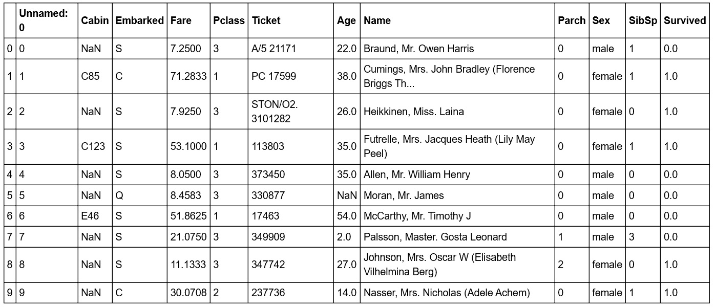
Figure 1.4: Reading the first 10 rows
Note
To access the source code for this specific section, please refer to https://packt.live/2Ynb7sf.
You can also run this example online at https://packt.live/2BvTRrG. You must execute the entire Notebook in order to get the desired result.
In this sample, we have a visual representation of the information in the DataFrame. We can see that the data is organized in a tabular, almost spreadsheet-like structure. The different types of data are organized into columns, while each sample is organized into rows. Each row is assigned an index value and is shown as the numbers 0 to 9 in bold on the left-hand side of the DataFrame. Each column is assigned to a label or name, as shown in bold at the top of the DataFrame.
The idea of a DataFrame as a kind of spreadsheet is a reasonable analogy. As we will see in this chapter, we can sort, filter, and perform computations on the data just as you would in a spreadsheet program. While it's not covered in this chapter, it is interesting to note that DataFrames also contain pivot table functionality, just like a spreadsheet (https://pandas.pydata.org/pandas-docs/stable/reference/api/pandas.pivot_table.html).
Exercise 1.02: Indexing and Selecting Data
Now that we have loaded some data, let's use the selection and indexing methods of the DataFrame to access some data of interest. This exercise is a continuation of Exercise 1.01, Loading and Summarizing the Titanic Dataset:
- Select individual columns in a similar way to a regular dictionary by using the labels of the columns, as shown here:
df['Age']
The output will be as follows:
0       22.0
1       38.0
2       26.0
3       35.0
4       35.0
        ...
1304     NaN
1305    39.0
1306    38.5
1307     NaN
1308     NaN
Name: Age, Length: 1309, dtype: float64
If there are no spaces in the column name, we can also use the dot operator. If there are spaces in the column names, we will need to use the bracket notation:
df.Age
The output will be as follows:
0 22.0 1 38.0 2 26.0 3 35.0 4 35.0 ... 1304 NaN 1305 39.0 1306 38.5 1307 NaN 1308 NaN Name: Age, Length: 1309, dtype: float64 - Select multiple columns at once using bracket notation, as shown here:
df[['Name', 'Parch', 'Sex']]
The output will be as follows:
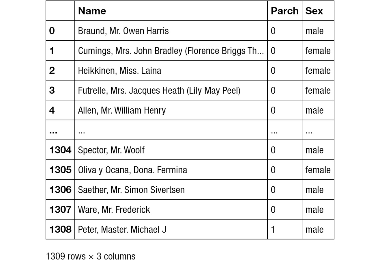
Figure 1.5: Selecting multiple columns
Note
The output has been truncated for presentation purposes.
- Select the first row using
iloc:df.iloc[0]
The output will be as follows:
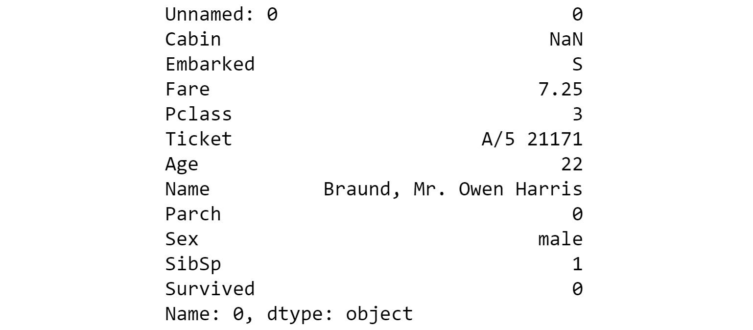
Figure 1.6: Selecting the first row
- Select the first three rows using
iloc:df.iloc[[0,1,2]]
The output will be as follows:
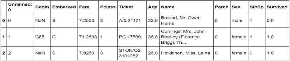
Figure 1.7: Selecting the first three rows
- Next, get a list of all of the available columns:
columns = df.columns # Extract the list of columns
print(columns)
The output will be as follows:

Figure 1.8: Getting all the columns
- Use this list of columns and the standard Python slicing syntax to get columns 2, 3, and 4, and their corresponding values:
df[columns[1:4]] # Columns 2, 3, 4
The output will be as follows:
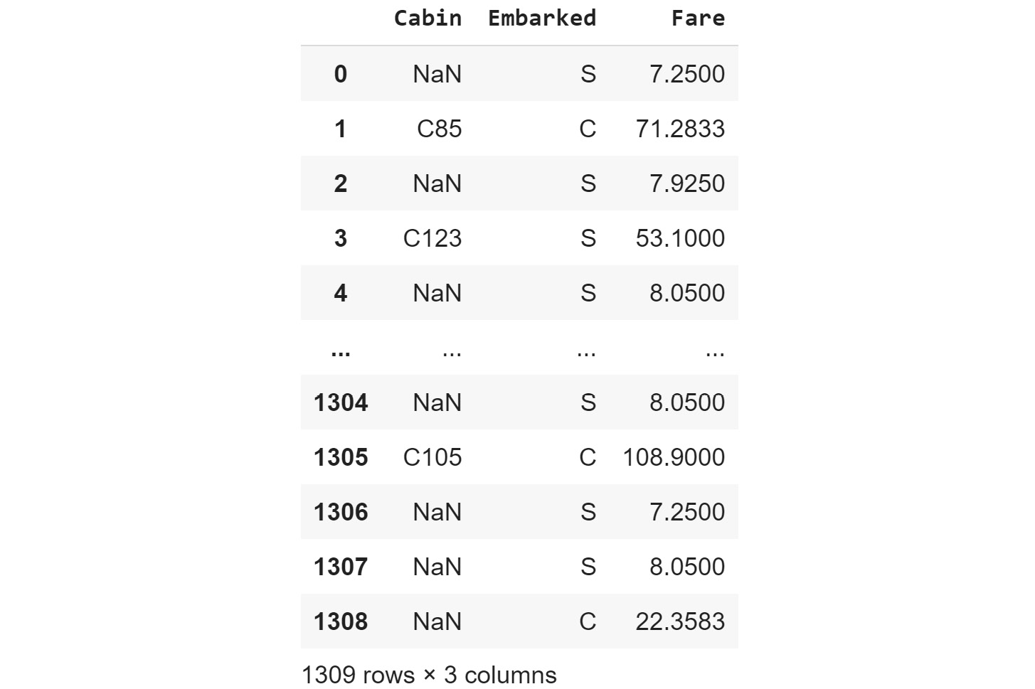
Figure 1.9: Getting the second, third, and fourth columns
- Use the
lenoperator to get the number of rows in the DataFrame:len(df)
The output will be as follows:
1309
- Get the value for the
Farecolumn in row 2 using the row-centric method:df.iloc[2]['Fare'] # Row centric
The output will be as follows:
7.925
- Use the dot operator for the column, as follows:
df.iloc[2].Fare # Row centric
The output will be as follows:
7.925
- Use the column-centric method, as follows:
df['Fare'][2] # Column centric
The output will be as follows:
7.925
- Use the column-centric method with the dot operator, as follows:
df.Fare[2] # Column centric
The output will be as follows:
7.925
Note
To access the source code for this specific section, please refer to https://packt.live/2YmA7jb.
You can also run this example online at https://packt.live/3dmk0qf. You must execute the entire Notebook in order to get the desired result.
In this exercise, we have seen how to use pandas' read_csv() function to load data into Python within a Jupyter notebook. We then explored a number of ways that pandas, by presenting the data in a DataFrame, facilitates selecting specific items in a DataFrame and viewing the contents. With these basics understood, let's look at some more advanced ways to index and select data.
Exercise 1.03: Advanced Indexing and Selection
With the basics of indexing and selection under our belt, we can turn our attention to more advanced indexing and selection. In this exercise, we will look at a few important methods for performing advanced indexing and selecting data. This exercise is a continuation of Exercise 1.01, Loading and Summarizing the Titanic Dataset:
- Create a list of the passengers' names and ages for those passengers under the age of 21, as shown here:
child_passengers = df[df.Age  < 21][['Name', 'Age']]
child_passengers.head()
The output will be as follows:
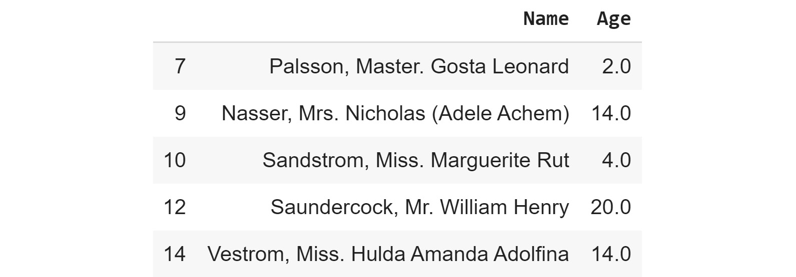
Figure 1.10: List of passengers' names and ages for those passengers under the age of 21
- Count how many child passengers there were, as shown here:
print(len(child_passengers))
The output will be as follows:
249
- Count how many passengers were between the ages of 21 and 30. Do not use Python's
andlogical operator for this step, but rather the ampersand symbol (&). Do this as follows:Note
The code snippet shown here uses a backslash (
\) to split the logic across multiple lines. When the code is executed, Python will ignore the backslash, and treat the code on the next line as a direct continuation of the current line.young_adult_passengers = df.loc[(df.Age > 21) \ & (df.Age < 30)] len(young_adult_passengers)
The output will be as follows:
279
- Find the passengers who were either first- or third-class ticket holders. Again, we will not use the Python logical
oroperator but the pipe symbol (|) instead. Do this as follows:df.loc[(df.Pclass == 3) | (df.Pclass ==1)]
The output will be as follows:
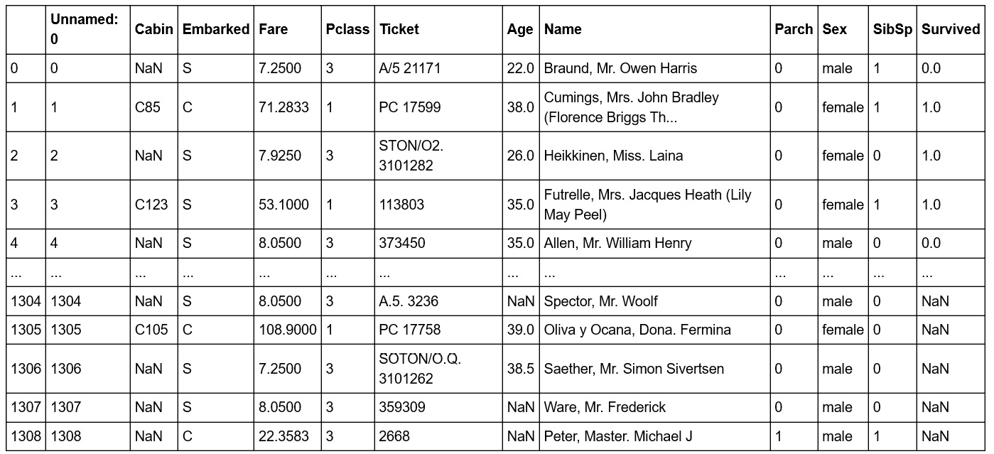
Figure 1.11: The number of passengers who were either first- or third-class ticket holders
- Find the passengers who were not holders of either first- or third-class tickets. Do not simply select those second-class ticket holders, but use the
~symbol for thenotlogical operator instead. Do this as follows:df.loc[~((df.Pclass == 3) | (df.Pclass == 1))]
The output will be as follows:
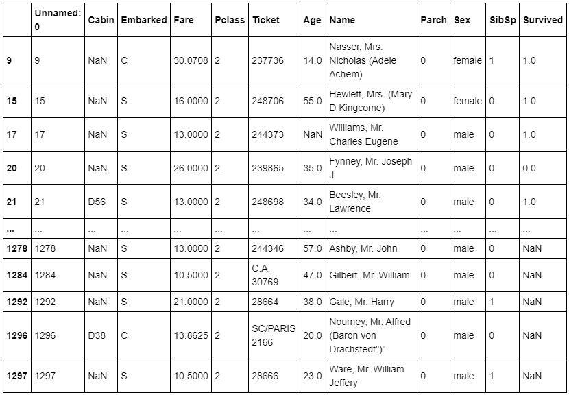
Figure 1.12: Count of passengers who were not holders of either first- or third-class tickets
- We no longer need the
Unnamed: 0column, so delete it using thedeloperator:del df['Unnamed: 0'] df.head()
The output will be as follows:
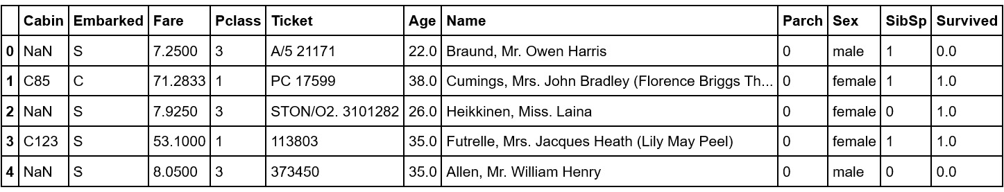
Figure 1.13: The del operator
Note
To access the source code for this specific section, please refer to https://packt.live/3empSRO.
You can also run this example online at https://packt.live/3fEsPgK. You must execute the entire Notebook in order to get the desired result.
In this exercise, we have seen how to select data from a DataFrame using conditional operators that inspect the data and return the subsets we want. We also saw how to remove a column we didn't need (in this case, the Unnamed column simply contained row numbers that are not relevant to analysis). Now, we'll dig deeper into some of the power of pandas.
Pandas Methods
Now that we are confident with some pandas basics, as well as some more advanced indexing and selecting tools, let's look at some other DataFrame methods. For a complete list of all methods available in a DataFrame, we can refer to the class documentation.
Note
The pandas documentation is available at https://pandas.pydata.org/pandas-docs/stable/reference/frame.html.
You should now know how many methods are available within a DataFrame. There are far too many to cover in detail in this chapter, so we will select a few that will give you a great start in supervised machine learning.
We have already seen the use of one method, head(), which provides the first five lines of the DataFrame. We can select more or fewer lines if we wish by providing the number of lines as an argument, as shown here:
df.head(n=20) # 20 lines
df.head(n=32) # 32 lines
Alternatively, you can use the tail() function to see a specified number of lines at the end of the DataFrame.
Another useful method is describe, which is a super-quick way of getting the descriptive statistics of the data within a DataFrame. We can see next that the sample size (count), mean, minimum, maximum, standard deviation, and the 25th, 50th, and 75th percentiles are returned for all columns of numerical data in the DataFrame (note that text columns have been omitted):
df.describe()
The output will be as follows:
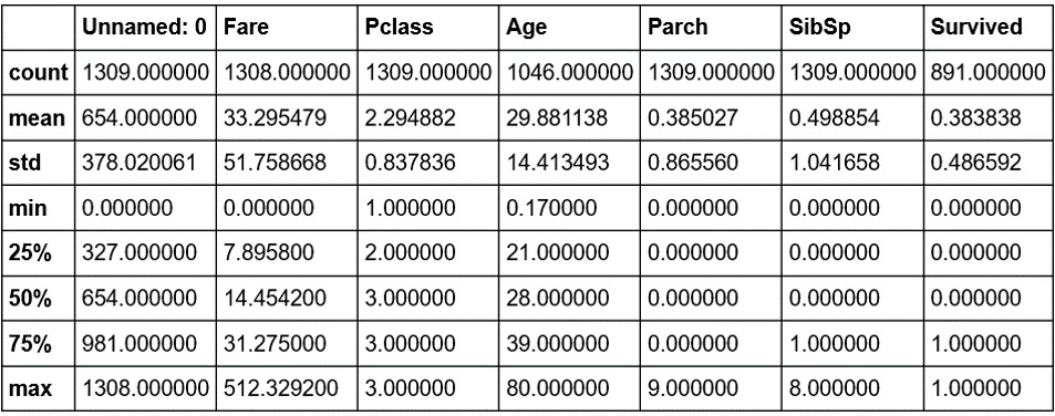
Figure 1.14: The describe method
Note that only columns of numerical data have been included within the summary. This simple command provides us with a lot of useful information; looking at the values for count (which counts the number of valid samples), we can see that there are 1,046 valid samples in the Age category, but 1,308 in Fare, and only 891 in Survived. We can see that the youngest person was 0.17 years, the average age is 29.898, and the eldest passenger was 80. The minimum fare was £0, with £33.30 the average and £512.33 the most expensive. If we look at the Survived column, we have 891 valid samples, with a mean of 0.38, which means about 38% survived.
We can also get these values separately for each of the columns by calling the respective methods of the DataFrame, as shown here:
df.count()
The output will be as follows:
Cabin        295
Embarked    1307
Fare        1308
Pclass      1309
Ticket      1309
Age         1046
Name        1309
Parch       1309
Sex         1309
SibSp       1309
Survived     891
dtype: int64
But we have some columns that contain text data, such as Embarked, Ticket, Name, and Sex. So what about these? How can we get some descriptive information for these columns? We can still use describe; we just need to pass it some more information. By default, describe will only include numerical columns and will compute the 25th, 50th, and 75th percentiles, but we can configure this to include text-based columns by passing the include = 'all' argument, as shown here:
df.describe(include='all')
The output will be as follows:
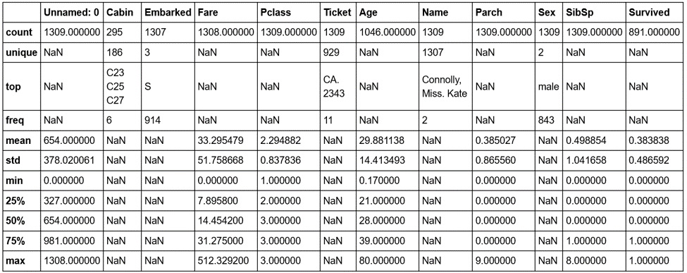
Figure 1.15: The describe method with text-based columns
That's better—now we have much more information. Looking at the Cabin column, we can see that there are 295 entries, with 186 unique values. The most common values are C32, C25, and C27, and they occur 6 times (from the freq value). Similarly, if we look at the Embarked column, we see that there are 1,307 entries, 3 unique values, and that the most commonly occurring value is S, with 914 entries.
Notice the occurrence of NaN values in our describe output table. NaN, or Not a Number, values are very important within DataFrames as they represent missing or not available data. The ability of the pandas library to read from data sources that contain missing or incomplete information is both a blessing and a curse. Many other libraries would simply fail to import or read the data file in the event of missing information, while the fact that it can be read also means that the missing data must be handled appropriately.
When looking at the output of the describe method, you should notice that the Jupyter notebook renders it in the same way as the original DataFrame that we read in using read_csv. There is a very good reason for this, as the results returned by the describe method are themselves a pandas DataFrame and thus possess the same methods and characteristics as the data read in from the CSV file. This can be easily verified using Python's built-in type function, as in the following code:
type(df.describe(include='all'))
The output will be as follows:
pandas.core.frame.DataFrame
Now that we have a summary of the dataset, let's dive in with a little more detail to get a better understanding of the available data.
Note
A comprehensive understanding of the available data is critical in any supervised learning problem. The source and type of the data, the means by which it is collected, and any errors potentially resulting from the collection process all have an effect on the performance of the final model.
Hopefully, by now, you are comfortable with using pandas to provide a high-level overview of the data. We will now spend some time looking into the data in greater detail.
Exercise 1.04: Using the Aggregate Method
We have already seen how we can index or select rows or columns from a DataFrame and use advanced indexing techniques to filter the available data based on specific criteria. Another handy method that allows for such selection is the groupby method, which provides a quick method for selecting groups of data at a time and provides additional functionality through the DataFrameGroupBy object. This exercise is a continuation of Exercise 1.01, Loading and Summarizing the Titanic Dataset:
- Use the
groupbymethod to group the data under theEmbarkedcolumn to find out how many different values forEmbarkedthere are:embarked_grouped = df.groupby('Embarked') print(f'There are {len(embarked_grouped)} Embarked groups')The output will be as follows:
There are 3 Embarked groups
- Display the output of
embarked_grouped.groupsto find what thegroupbymethod actually does:embarked_grouped.groups
The output will be as follows:
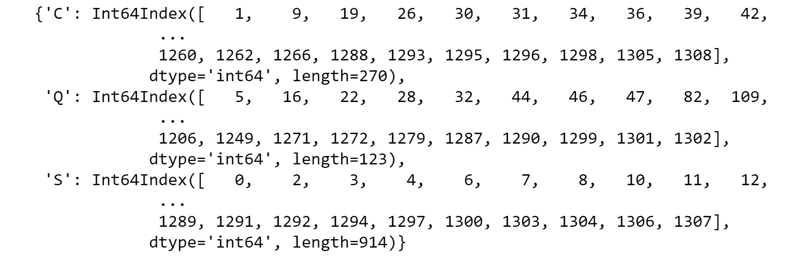
Figure 1.16: Output of embarked_grouped.groups
We can see here that the three groups are
C,Q, andS, and thatembarked_grouped.groupsis actually a dictionary where the keys are the groups. The values are the rows or indexes of the entries that belong to that group. - Use the
ilocmethod to inspect row1and confirm that it belongs to embarked groupC:df.iloc[1]
The output will be as follows:
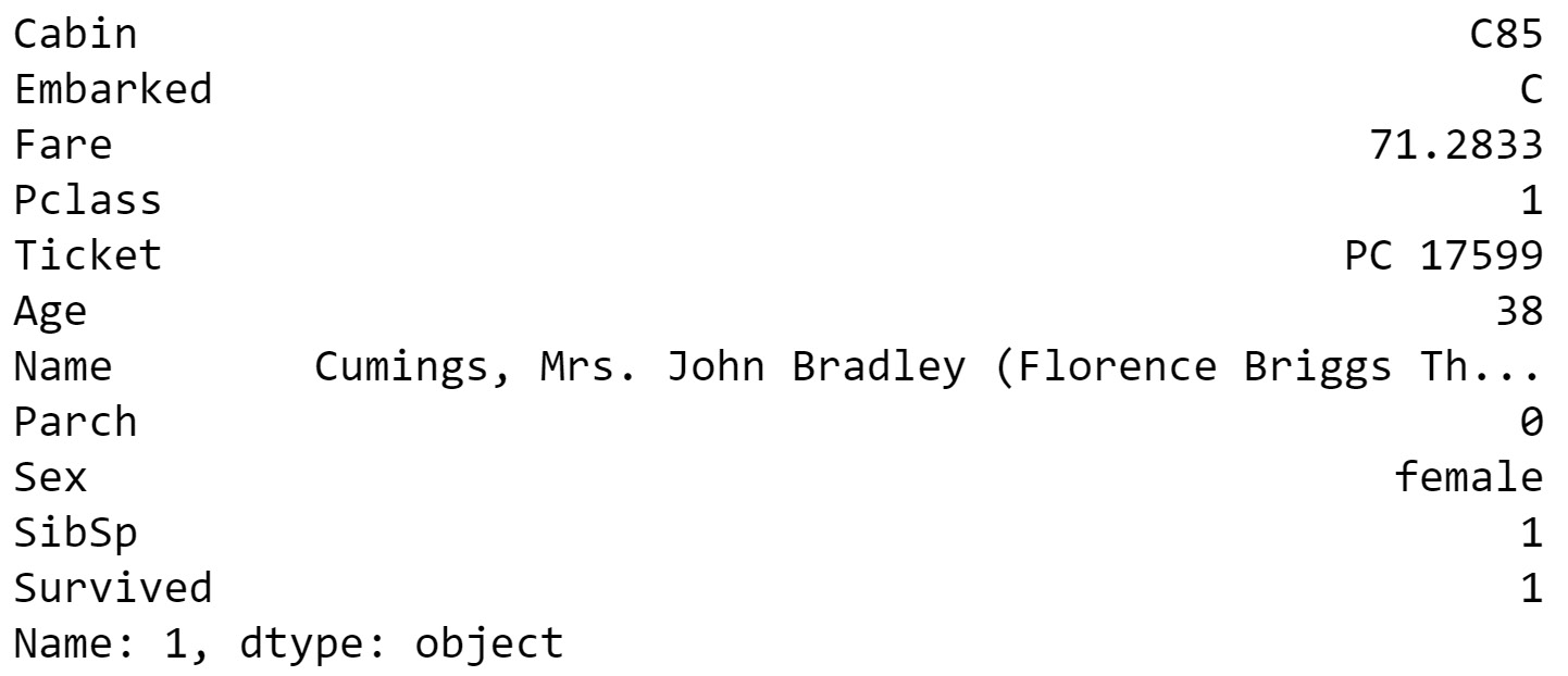
Figure 1.17: Inspecting row 1
- As the groups are a dictionary, we can iterate through them and execute computations on the individual groups. Compute the mean age for each group, as shown here:
for name, group in embarked_grouped:
    print(name, group.Age.mean())
The output will be as follows:
C 32.33216981132075
Q 28.63
S 29.245204603580564
- Another option is to use the
aggregatemethod, oraggfor short, and provide it with the function to apply across the columns. Use theaggmethod to determine the mean of each group:embarked_grouped.agg(np.mean)
The output will be as follows:
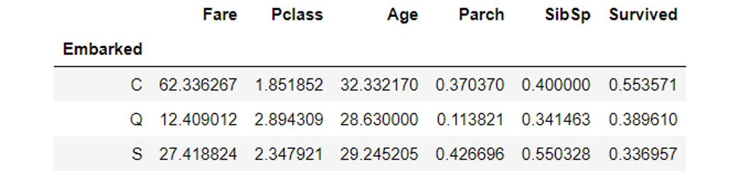
Figure 1.18: Using the agg method
So, how exactly does
aggwork and what type of functions can we pass it? Before we can answer these questions, we need to first consider the data type of each column in the DataFrame, as each column is passed through this function to produce the result we see here. Each DataFrame comprises a collection of columns of pandas series data, which, in many ways, operates just like a list. As such, any function that can take a list or a similar iterable and compute a single value as a result can be used withagg. - Define a simple function that returns the first value in the column and then pass that function through to
agg, as an example:def first_val(x): return x.values[0] embarked_grouped.agg(first_val)
The output will be as follows:
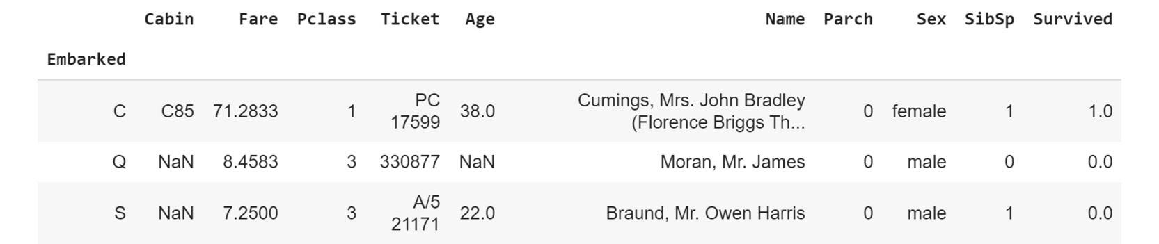
Figure 1.19: Using the .agg method with a function
Note
To access the source code for this specific section, please refer to https://packt.live/2NlEkgM.
You can also run this example online at https://packt.live/2AZnq51. You must execute the entire Notebook in order to get the desired result.
In this exercise, we have seen how to group data within a DataFrame, which then allows additional functions to be applied using .agg(), such as to calculate group means. These sorts of operations are extremely common in analyzing and preparing data for analysis.
Quantiles
The previous exercise demonstrated how to find the mean. In statistical data analysis, we are also often interested in knowing the value in a dataset below or above which a certain fraction of the points lie. Such points are called quantiles. For example, if we had a sequence of numbers from 1 to 10,001, the quantile for 25% is the value 2,501. That is, at the value 2,501, 25% of our data lies below that cutoff. Quantiles are often used in data visualizations because they convey a sense of the distribution of the data. In particular, the standard boxplot in Matplotlib draws a box bounded by the first and third of 4 quantiles.
For example, let's establish the 25% quantile of the following dataframe:
import pandas as pd
df = pd.DataFrame({"A":[1, 6, 9, 9]})
#calculate the 25% quantile over the dataframe
df.quantile(0.25, axis = 0)
The output will be as follows:
A    4.75
Name: 0.25, dtype: float64
As you can see from the preceding output, 4.75 is the 25% quantile value for the DataFrame.
Note
For more information on quantile methods, refer to https://pandas.pydata.org/pandas-docs/stable/reference/frame.html.
Later in this book, we'll use the idea of quantiles as we explore the data.
Lambda Functions
One common and useful way of implementing agg is through the use of Lambda functions.
Lambda, or anonymous, functions (also known as inline functions in other languages) are small, single-expression functions that can be declared and used without the need for a formal function definition via the use of the def keyword. Lambda functions are essentially provided for convenience and aren't intended to be used for extensive periods. The main benefit of Lambda functions is that they can be used in places where a function might not be appropriate or convenient, such as inside other expressions or function calls. The standard syntax for a Lambda function is as follows (always starting with the lambda keyword):
lambda <input values>: <computation for values to be returned>
Let's now do an exercise and create some interesting Lambda functions.
Exercise 1.05: Creating Lambda Functions
In this exercise, we will create a Lambda function that returns the first value in a column and use it with agg. This exercise is a continuation of Exercise 1.01, Loading and Summarizing the Titanic Dataset:
- Write the
first_valfunction as a Lambda function, passed toagg:embarked_grouped = df.groupby('Embarked') embarked_grouped.agg(lambda x: x.values[0])The output will be as follows:
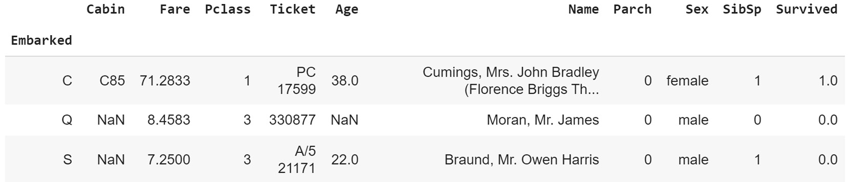
Figure 1.20: Using the agg method with a Lambda function
Obviously, we get the same result, but notice how much more convenient the Lambda function was to use, especially given the fact that it is only intended to be used briefly.
- We can also pass multiple functions to
aggvia a list to apply the functions across the dataset. Pass the Lambda function as well as the NumPy mean and standard deviation functions, like this:embarked_grouped.agg([lambda x: x.values[0], np.mean, np.std])
The output will be as follows:
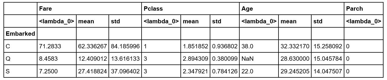
Figure 1.21: Using the agg method with multiple Lambda functions
- Apply
numpy.sumto theFarecolumn and the Lambda function to theAgecolumn by passingagga dictionary where the keys are the columns to apply the function to, and the values are the functions themselves to be able to apply different functions to different columns in the DataFrame:embarked_grouped.agg({'Fare': np.sum, \ 'Age': lambda x: x.values[0]})The output will be as follows:

Figure 1.22: Using the agg method with a dictionary of different columns
- Finally, execute the
groupbymethod using more than one column. Provide the method with a list of the columns (SexandEmbarked) togroupby, like this:age_embarked_grouped = df.groupby(['Sex', 'Embarked']) age_embarked_grouped.groups
The output will be as follows:
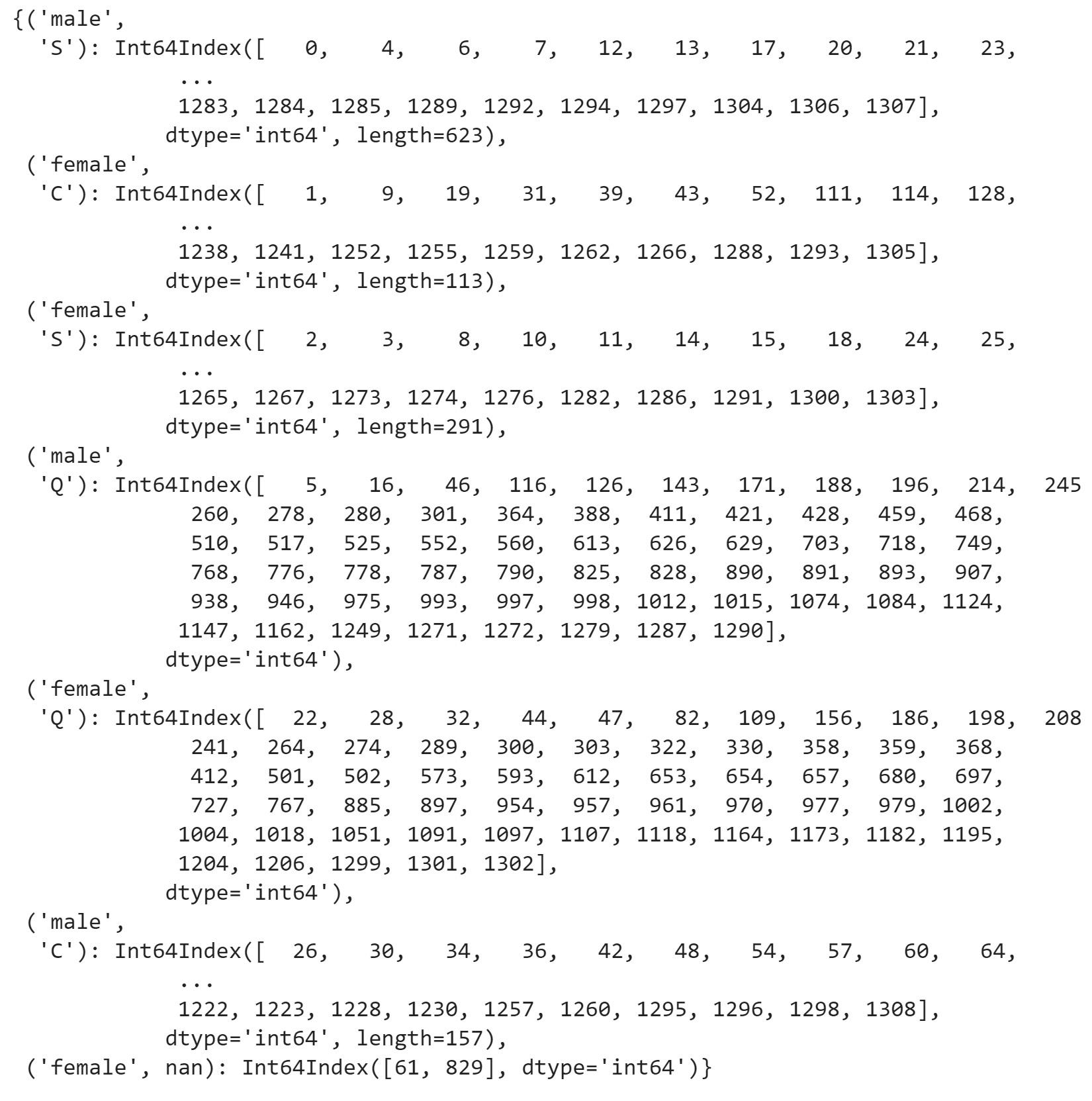
Figure 1.23: Using the groupby method with more than one column
Similar to when the groupings were computed by just the Embarked column, we can see here that a dictionary is returned where the keys are the combination of the Sex and Embarked columns returned as a tuple. The first key-value pair in the dictionary is a tuple, ('Male', 'S'), and the values correspond to the indices of rows with that specific combination. There will be a key-value pair for each combination of unique values in the Sex and Embarked columns.
Note
To access the source code for this specific section, please refer to https://packt.live/2B1jAZl.
You can also run this example online at https://packt.live/3emqwPe. You must execute the entire Notebook in order to get the desired result.
This concludes our brief exploration of data inspection and manipulation. We now move on to one of the most important topics in data science, data quality.