Data Manipulation

Now that we have deconstructed the structure of the pandas DataFrame down to its basics, the remainder of the wrangling tasks, that is, creating new DataFrames, selecting or slicing a DataFrame into its parts, filtering DataFrames for some values, joining different DataFrames, and so on, will become very intuitive. Let's start by selecting and filtering in the following section.

Note

Jupyter notebooks for the code examples listed in this chapter can be found at the following links: https://packt.link/xTvR2 and https://packt.link/PGIzK.

Selecting and Filtering in pandas

If you wanted to access a particular cell in a spreadsheet, you would do so by addressing that cell in the familiar format of (column name, row name). For example, when you call cell A63, A refers to the column and 63 refers to the row. Data is stored similarly in pandas, but as (row name, column name) and we can use the same convention to access cells in a DataFrame.

For example, look at the following DataFrame. The viewers column is the index of the DataFrame:

Figure 1.23: Sample DataFrame

To find the cost of acquisition of Adam and Anurag along with their views, we can use the following code. Here, Adam and Anurag are the rows, and cost, along with views, are the columns:

df.loc[['Adam','Anurag'],['cost','views']]

Running the preceding command will generate the following output:

Figure 1.24: Use of the loc function

If you need to access more than a single cell, such as a subset of some rows and columns from the DataFrame, or change the order of display of some columns on the DataFrame, you can make use of the syntax listed in the following table:

Figure 1.25: A table listing the syntax used for different operations on a pandas DataFrame

In the next section, you'll learn how to create DataFrames in Python.

Creating DataFrames in Python

Let's say you've loaded campaign data into a DataFrame. In the revenue column, you see that the figures are not in their desired currencies. To convert the revenue numbers to various other currencies, you may need to create a test DataFrame, containing exchange rates that will remain constant throughout your revenue calculation.

There are two ways of creating such test DataFrames—by creating completely new DataFrames, or by duplicating or taking a slice of a previously existing DataFrame:

• Creating new DataFrames: You typically use the DataFrame function to create a completely new DataFrame. The function directly converts a Python object into a pandas DataFrame. The DataFrame function in general works with any iterable collection of data, such as dict and list. You can also pass an empty collection or a singleton collection to it.

  For example, you will get the same DataFrame through either of the following lines of code:

  df=pd.DataFrame({'Currency': pd.Series(['USD','EUR','GBP']),\

                   'ValueInINR': pd.Series([70, 89, 99])})

  df=pd.DataFrame.from_dict({'Currency': ['USD','EUR','GBP'],\

                             'ValueInINR':[70, 89, 99]})

  df.head()

  Running the command in either of these two ways will generate the following output:

  

Figure 1.26: Output generated by two different ways to create a DataFrame

• Duplicating or slicing a previously existing DataFrame: The second way to create a DataFrame is by copying a previously existing DataFrame. Your first intuition would be to do something like obj1 = obj2. However, since both the objects share a reference to the same object in memory, changing obj2 will also change obj1, and vice versa.

  You can tackle this with a standard library function called deepcopy. The deepcopy function allows the user to recursively go through the objects being pointed to by the references and create entirely new objects.

  So, when you want to copy a previously existing DataFrame and don't want the previous DataFrame to be affected by modifications in the new DataFrame, you need to use the deepcopy function. You can also slice the previously existing DataFrame and pass it to the function, and it will be considered a new DataFrame.

  For example, the following code snippet will recursively copy everything in df (refer Figure 1.26) to df1. Now, any changes you make to df1 won't have an impact on df:

  import pandas

  import copy

  df1 = df.copy(deep=True)

  The contents of df1 will be the same as what we see in Figure 1.26.

In the next section, you will look at functions that can help you to add or remove attributes in a pandas DataFrame.

Adding and Removing Attributes and Observations

pandas provides the following functions to add and delete rows (observations) and columns (attributes):

• df['col'] = s: This adds a new column, col, to the DataFrame, df, creating a new column that has values from the series, s.
• df.assign(c1 = s1, c2 = s2...): This method adds new columns, c1, c2, and so on, with series, s1, s2, and so on, to the df DataFrame in one go.
• df.append(df2): This method adds values from the df2 DataFrame to the bottom of the df DataFrame wherever the columns of df2 match those of df.
• df.drop(labels, axis): This method removes the rows or columns specified by the labels and corresponding axis, or those specified by the index or column names directly.

  For example, in the DataFrame created in Figure 1.26, if we wanted to drop the Currency column, the corresponding code would be as follows:

  df=df.drop(['Currency'],axis=1)

  The output should be as follows:

  

Figure 1.27: Output when the Currency column is dropped from the df DataFrame

• df.dropna(axis, how): Depending on the parameter passed to how, this method decides whether to drop rows (or columns if axis = 1) with missing values in any of the fields or in all of the fields. If no parameter is passed, the default value of how is any, and the default value of the axis is 0.
• df.drop_duplicates(keep): This method removes rows with duplicate values in the DataFrame, and keeps the first (keep = 'first'), last (keep = 'last'), or no occurrence (keep = False) in the data.

DataFrames can also be sequentially combined with the concat function:

• pd.concat([df1,df2..]): This method creates a new DataFrame with df1, df2, and all other DataFrames combined sequentially. It will automatically combine columns having the same names in the combined DataFrames.

In the next section, you will learn how to combine data from different DataFrames into a single DataFrame.

Combining Data

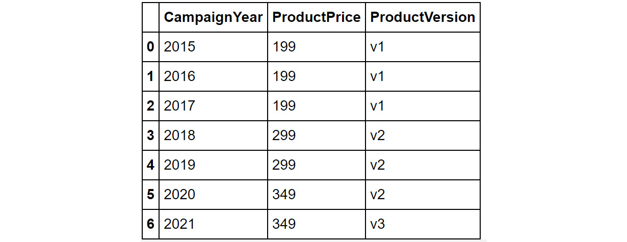
Let's say the product team sends you details about the prices of the popular products your company makes. The data is stored in a DataFrame called df_products and contains the following information:

Figure 1.28: Contents of the df_products DataFrame

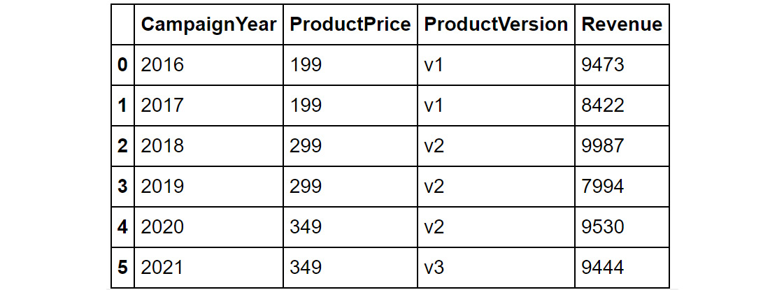
The finance team has also sent you details regarding the revenue for these products, stored in a DataFrame called df_revenue. It contains the following details:

Figure 1.29: Contents of the df_revenue DataFrame

Notice that in both these DataFrames, the CampaignYear column is common; however, since the finance team didn't have details of the 2015 campaign, that entry is missing in the df_revenue DataFrame. Now, let's say you wanted to combine data from both these DataFrames into a single DataFrame. The easiest way you'd go about this is to use the pd.merge function:

df_combined = pd.merge(df_products, df_revenue)

Note

In the preceding code, df_products is considered the left DataFrame, while df_revenue is considered the right DataFrame.

The contents of the combined DataFrame should look as follows:

Figure 1.30: Contents of the merged DataFrame

As you can see from the output in Figure 1.30, the DataFrames are merged on the common column (which is CampaignYear). One thing you'll notice is that the data for CampaignYear 2015 is missing. To make sense of this phenomenon, let's understand what is happening behind the scenes.

When we ran the merge() command, pandas merged df_products and df_revenue based on a common column in the two datasets – this was CampaignYear. If there were multiple shared columns in the two datasets, we'd have to specify the exact column we want to merge on as follows:

df_combined = pd.merge(df_products, df_revenue, \

                       on = "CampaignYear")

Now, since the CampaignYear column is the only column shared between the two DataFrames and the entry for 2015 is missing in one of the DataFrames (and hence not a shared value), it is excluded in the combined dataset.

What if we still wanted to examine the price and version of the product for 2015 and have revenue as blank for that year? We can fine-tune the merging of DataFrames by using the how parameter.

With the help of the how parameter, you can merge DataFrames in four different  ways:

Figure 1.31: Table describing different joins

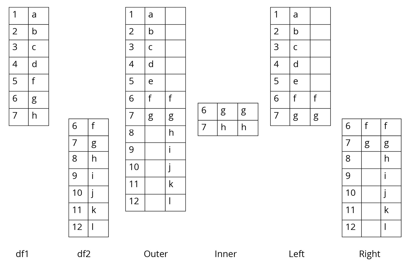
The following diagram shows two sample DataFrames, df1 and df2, and the results of the various joins performed on these DataFrames:

Figure 1.32: Table showing two DataFrames and the outcomes of different joins on them

In the preceding diagram, outer join returns all the records in df1 and df2 irrespective of a match (any missing values are filled with NaN entries). For example, if we wanted to do an outer join with the products and revenue DataFrames, we would have to run the following command:

df_combined_outer = pd.merge(df_products, df_revenue, \

                             how = 'outer')

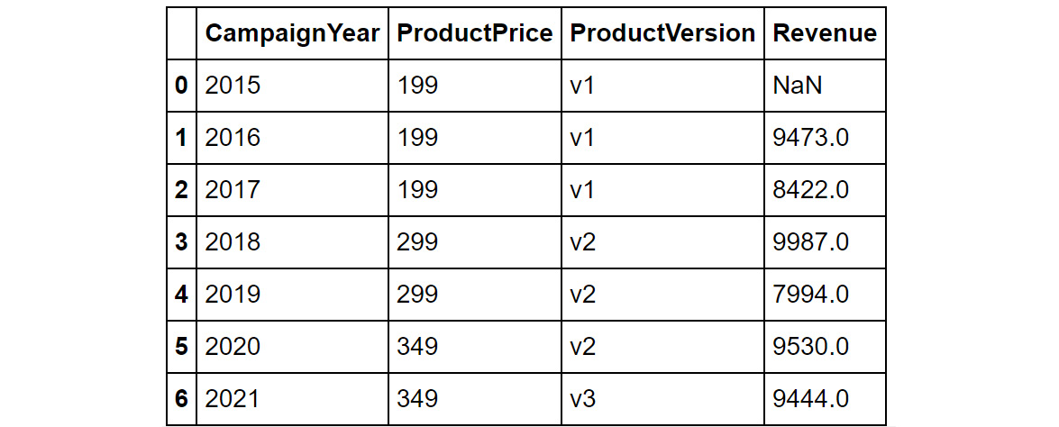
The output should be as follows:

Figure 1.33: Outer join

You can see that with outer join, even the row that did not match (2015) is included.

Inner join returns records with matching values in df1 and df2. From Figure 1.32, you can see that those are 6 and 7. If you merged the products and revenue DataFrames using an inner join, you'd have the same output that you see in Figure 1.33. By default, pandas uses an inner join.

Left join returns all the records in the left DataFrame and the matched records in the right DataFrame. If any values are missing, it will fill those entries with NaN values. In the products and revenue DataFrames, a left join on the CampaignYear column would return even the row representing 2015, except that the entry for revenue would be NaN.

Right join works similar to left join, except that it returns all the records from the right DataFrame along with just the matching records from the left DataFrame.

So far, you have seen how to merge DataFrames with the same column names. But what if you tried to merge DataFrames containing common data but with differently named columns? In such cases, you will have to specify the column names of the left and the right DataFrame as follows:

df_combined_specific = pd.merge(df_products, df_revenue, \

                               left_on="CampaignYear", \

                               right_on="CampaignYear2")

In the preceding code block, left_on specifies the column name of the left DataFrame (df_products), while right_on specifies the column name of the right DataFrame (df_revenue).

You have seen how to join DataFrames in this section. In the next section, you will be looking at how to handle missing values.

Handling Missing Data

As a marketing analyst, you will encounter data with missing values quite a lot. For example, let's say you join a Product category table with an Ad viewership table. Upon merging these two, you may find that not all product categories will have a corresponding value in the Ad Viewership table. For example, if a company ran no ads for winter clothes in tropical countries, values for those products in the Ad Viewership table would be missing. Such instances are quite common when dealing with real-world data.

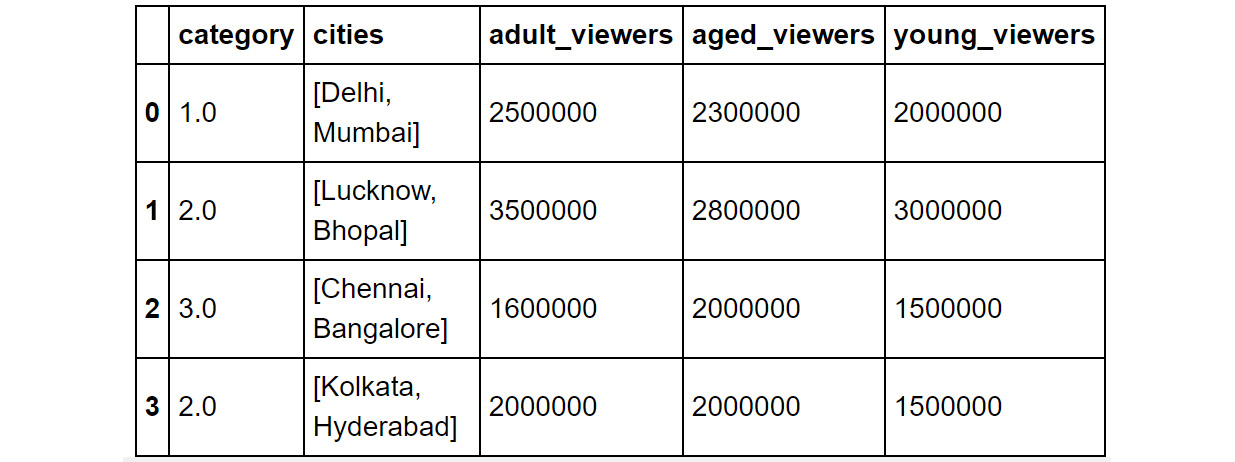
Here's another example of missing data where the category column in the DataFrame has a missing value (demarcated by NaN):

Figure 1.34: Sample DataFrame

While the way you can treat missing values varies based on the position of the missing values and the particular business use case, here are some general strategies that you can employ:

• You can get rid of missing values completely using df.dropna, as explained in the Adding and Removing Attributes and Observations section previously.
• You can also replace all the missing values simultaneously using df.fillna().

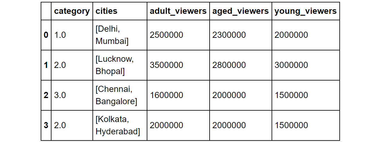
When using fillna(), the value you want to fill in will depend heavily on the context and the use case for the data. For example, you can replace all missing values with the mean of the column where the missing value is present:

df.fillna(df.mean())

You should then get the following output:

Figure 1.35: Output of the df.fillna(df.mean()) command

Or the median of the data, as in this example:

df.fillna(df.median())

You should then get the following output:

Figure 1.36: Output of the df.fillna(df.median()) command

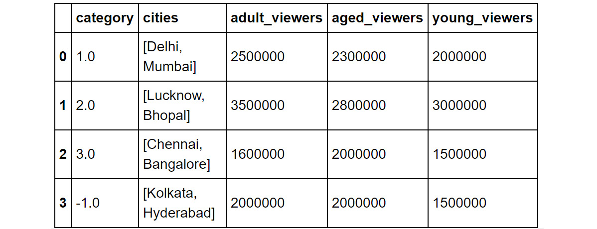
Or, with some values, such as –1 (or any number of your choice) if you want the record to stand apart during your analysis:

df.fillna(-1)

You should then get the following output:

Figure 1.37: Using the df.fillna function

To help deal with missing values better, there are some other built-in functions you can use. These will help you quickly check whether your DataFrame contains any missing values.

You can check for slices containing missing values using the isnull() function:

df.isnull()

This command will return output like the following:

Figure 1.38: Using the .isnull function

The entries where there are null values will show up as True. If not, they'll show up as False.

Similarly, you can check whether individual elements are NA using the isna function. Here, we are using the isna function with the category column:

df[['category']].isna

The command will provide you with a Boolean output. True means that the element is null, and False means it is not:

Figure 1.39: Using the isna function used on a column

In the next exercise, you will be combing different DataFrames and taking care of the missing values.

Exercise 1.03: Combining DataFrames and Handling Missing Values

As part of its forthcoming holiday campaign, the business wanted to understand the cost of acquisition of customers for an e-commerce website specializing in kids' toys. As a marketing analyst, you now have to dig through the historical records of the previous campaign and suggest the marketing budget for the current campaign.

In this exercise, you will be importing two CSV files, timeSpent.csv and cost.csv, into the DataFrames df1 and df2. The df1 DataFrame has the details of the users, along with the time spent on the website. The df2 DataFrame consists of the cost of acquisition of a user.

You will combine the DataFrame containing the time spent by the users with the other DataFrame containing the cost of acquisition of the user. You will merge both these DataFrames to get an idea of user behavior.

Perform the following steps to achieve the aim of this exercise:

1. Import the pandas modules that you will be using in this exercise:

   import pandas as pd

2. Load the CSV files into the DataFrames df1 and df2:

   df1 =pd.read_csv("timeSpent.csv")

   df2 =pd.read_csv("cost.csv")

   Note

   You can find the timeSpent.csv file at https://packt.link/bpfVk and the cost.csv file at https://packt.link/pmpkK.

   Also, do make sure that you modify the path (emboldened) based on where these files are saved on your system.

3. Examine the first few rows of the first DataFrame using the head() function:

   df1.head()

   You should get the following output:

   

   Figure 1.40: Contents of df1

   You can see that the DataFrame, df1, has two columns – users and timeSpent.

4. Next, look at the first few rows of the second dataset:

   df2.head()

   You should get the following output:

   

   Figure 1.41: Contents of df2

   As you can see, DataFrame df2 has two columns – users and cost. In the cost column, there is a NaN value.

5. Do a left join of df1 with df2 and store the output in a DataFrame, df. Use a left join as we are only interested in users who are spending time on the website. Specify the joining key as "users":

   df = df1.merge(df2, on="users", how="left")

   df.head()

   Your output should now look as follows:

   

   Figure 1.42: Using the merge and fillna functions

6. You'll observe some missing values (NaN) in the preceding output. These types of scenarios are very common as you may fail to capture some details pertaining to the users. This can be attributed to the fact that some users visited the website organically and hence, the cost of acquisition is zero.

   These missing values can be replaced with the value 0. Use the following code:

   df=df.fillna(0)

   df.head()

   Your output should now look as follows:

   

Figure 1.43: Imputing missing values with the fillna function

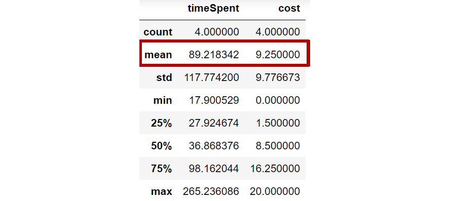
Now, the DataFrame has no missing values and you can compute the average cost of acquisition along with the average time spent. To compute the average value, you will be using the built-in function describe, which gives the statistics of the numerical columns in the DataFrame. Run the following command:

df.describe()

You should then get the following result:

Figure 1.44: Mean value of the columns

From the preceding screenshot, you can infer that the average cost of acquisition of a user is $9.25 and, on average, a user spends around 89 seconds on the website. Based on the traffic you want to attract for the forthcoming holiday season, you can now compute the marketing budget using the following formula:

Marketing Budget = Number of users * Cost of Acquisition

In this exercise, you have successfully dealt with missing values in your data. Do keep in mind that handling missing values is more of an art than science and each scenario might be different. In the next section, you will learn how to apply functions and operations on a DataFrame.

Applying Functions and Operations on DataFrames

By default, operations on all pandas objects are element-wise and return the same type of pandas objects. For instance, look at the following code:

df['viewers'] = df['adult_viewers']\

                +df['aged_viewers']+df['young_viewers']

The preceding code will add a viewers column to the DataFrame, with the value for each observation equaling the sum of the values in the adult_viewers, aged_viewers, and young_viewers columns.

Similarly, the following code will multiply every numerical value in the viewers column of the DataFrame by 0.03 or whatever value you want to keep as your target CTR (click-through rate):

df['expected clicks'] = 0.03*df['viewers']

Hence, your DataFrame will look as follows once these operations have been performed:

Figure 1.45: Operations on pandas DataFrames

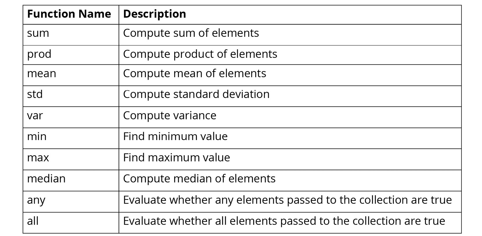
pandas also supports several built-in functions on pandas objects:

Figure 1.46: Built-in functions used in pandas

Note

Remember that pandas objects are Python objects, too. Therefore, you can write your custom functions to perform specific tasks on them.

To apply built-in or custom functions to pandas, you can make use of the map and apply functions. You can pass any built-in, NumPy, or custom functions as parameters to these functions and they will be applied to all elements in the column:

• map: map executes a function on each value present in the column. For example, look at the following DataFrame:

Figure 1.47: A sample DataFrame

Now, suppose you want to change the values of the Gender column to denote Female as F and Male as M. This can be achieved with the help of the map function. You'll need to pass values to the map function in the form of a dictionary:

df['Gender']=df['Gender'].map({"Female":"F","Male":"M"})

You should get the following result:

Figure 1.48: Using the map function

In the preceding screenshot, you can see that the values in the Gender column are now displayed as M and F.

• apply: This applies the function to the object passed and returns a DataFrame. It can easily take multiple columns as input. It also accepts the axis parameter, depending on how the function is to be applied. For example, let's say in the following DataFrame you wanted to sum all the purchases made by the user across the different categories and store the sum in a new column:

Figure 1.49: Sample DataFrame

You can achieve this with the help of the apply function as follows:

df1['purchase']=df1[['electronics','food','furniture']]\

                .apply(np.sum,axis=1)

df1

Note

In the preceding code, since you're using NumPy, you will need to import the numpy library before trying out the code. You can do so by using import numpy as np.

You should then get the following result:

Figure 1.50: Using the apply function

In the preceding screenshot, you can see that a new column, purchase, is created, which is the sum of the electronics, food, and furniture columns.

In this section, you have learned how to apply functions and operations to columns and rows of a DataFrame. In the next section, you will look at how to group data.

Grouping Data

Let's suppose, based on certain conditions, that you wanted to apply a function to multiple rows of a DataFrame. For example, you may need to do so when you want to calculate the sum of product prices separately for each currency. The pythonic way to solve this problem is to slice the DataFrame on the key(s) you want to aggregate on and then apply your function to that group, store the values, and move on to the next group. pandas provides a better way to do this, using the groupby function.

Let's look at the following DataFrame:

Figure 1.51: Sample DataFrame

If you want to find out the total cost of acquisition based on gender, you can use the following code:

df.groupby('Gender')['cost'].sum()

You should then get the following output:

Figure 1.52: Using the groupby function

In the preceding screenshot, you can see that the male users have a higher cost of acquisition than female users. In the next exercise, you will implement some of the operations you have learned so far.

Exercise 1.04: Applying Data Transformations

In Exercise 1.01, Loading Data Stored in a JSON File, you worked with a JSON file that contained the details of the users of a shopping app. There, your task was to validate whether the data was loaded correctly and to provide some answers about the information contained in it. Since you confirmed that the data was loading correctly, you'll be working with the same dataset once again, but this time, you'll be analyzing the underlying data. Also, this time, you'll be answering some interesting questions that the marketing team has come up with:

• What is the average age of the users?
• Which is the favorite fruit of the users?
• Do you have more female customers?
• How many of the users are active?

This exercise aims to get you used to performing regular and groupby operations on DataFrames and applying functions to them. You will use the user_info.json file on GitHub.

Note

You can find the user_info.json file at the following link: https://packt.link/Gi2O7.

1. Import the pandas module using the following command:

   import pandas as pd

2. Read the user_info.json file into a pandas DataFrame, user_info, using the following command:

   user_info = pd.read_json('user_info.json')

   Note

   Make sure you change the path (emboldened) to the JSON file based on its location on your system. If you're running the Jupyter notebook from the same directory where the JSON file is stored, you can run the preceding code without any modification.

3. Now, examine whether your data is properly loaded by checking the first few values in the DataFrame. Do this using the head() command:

   user_info.head()

   You should get the following output:

   

   Figure 1.53: Output of the head function on user_info

   Note

   Not all columns and rows are shown in the preceding output.

   The data consists of session information of the customers, along with their demographic details, contact information, and other details.

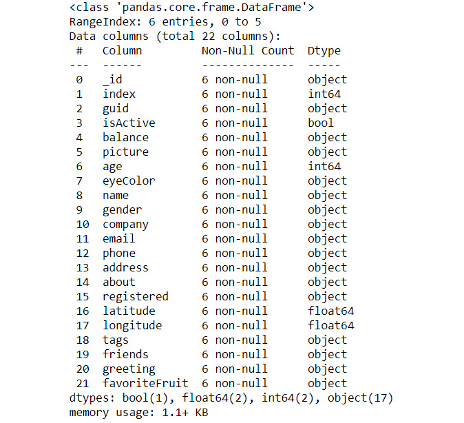
4. Now, look at the attributes and the data inside them using the following command:

   user_info.info()

   You should get the following output:

   

   Figure 1.54: Output of the info function on user_info

5. Now, let's start answering the questions:

   What is the average age of the users? To find the average age, use the following code:

   user_info['age'].mean()

   You will get the output as 27.83, which means that the average age of the users is 27.83.

   Which is the favorite fruit among the users? To answer this question, you can use the groupby function on the favoriteFruit column and get a count of users with the following code:

   user_info.groupby('favoriteFruit')['_id'].count()

   You should get the following output:

   

Figure 1.55: Output of the count function

From the preceding screenshot, you can see that there is no clear winner as both apple and strawberry have the same count of 3.

Do you have more female customers? To answer this question, you need to count the number of male and female users. You can find this count with the help of the groupby function. Use the following code:

user_info.groupby('gender')['_id'].count()

You should get the following output:

Figure 1.56: Output of the count function

From the preceding screenshot, you can infer that you have an equal split of customers concerning gender. Now, let's move on to our last question.

How many of the users are active? Similar to the preceding questions, you can use the groupby function on the isActive column to find out the answer.

Use the following code:

user_info.groupby('isActive')['_id'].count()

You should get the following output:

Figure 1.57: Output of the count function

From the preceding screenshot, you see that three customers are active while the other three are inactive.

This exercise acts as a short introduction to applying data transformations, functions, and getting an overview of aggregation, which can come in handy during the exploratory phase of a project.

Now that you have learned the different aspects of data preparation and cleaning, let's test your skills with the help of the following activity.

Activity 1.01: Addressing Data Spilling

The data we receive in most cases is not clean. There will be issues such as missing values, incorrect data types, data not loaded properly in the columns, and more. As a marketing analyst, you will have to clean this data and render it in a usable format so that you can analyze it further to mine useful information.

In this activity, you will now solve the problem that you encountered in Exercise 1.02, Loading Data from Multiple Sources. You will start by loading sales.csv, which contains some historical sales data about different customer purchases in stores in the past few years. As you may recall, the data loaded in the DataFrame was not correct as the values of some columns were getting populated wrongly in other columns. The goal of this activity is to clean the DataFrame and make it into a usable form.

You need to read the files into pandas DataFrames and prepare the output so that it can be used for further analysis. Follow the steps given here:

1. Open a new Jupyter notebook and import the pandas module.
2. Load the data from sales.csv into a separate DataFrame, named sales, and look at the first few rows of the generated DataFrame.

   Note

   You can find the sales.csv file at https://packt.link/IDGB4.

   You should get the following output:

   

   Figure 1.58: Output of the head function on sales.csv

3. Analyze the data type of the fields.
4. Look at the first column. If the value in the column matches the expected values, move on to the next column or otherwise fix it with the correct value.
5. Once you have fixed the first column, examine the other columns one by one and try to ascertain whether the values are right.

   Hint

   As per the information from the product team, the file contains information about their product line, which is camping equipment, along with information about their flagship product.

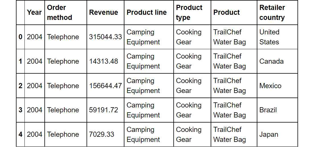
   Once you have cleaned the DataFrame, your final output should appear as follows:

   

Figure 1.59: First few rows of the structured DataFrame

Note

The solution to this activity can be found via this link.