Introducing models, datasets, and supervised learning

In the previous section, we introduced a model as a construct to replace a set of instructions that typically comprise a program to perform a specific task. This section covers models and other core machine learning concepts in more detail.

Models

More formally, a model is a mathematical or algorithmic representation of a specific process that performs a particular task. A machine learning model learns a particular task by being trained on a dataset using a training algorithm.

Note

An alternative term for training is fit. Historically, fit stems from the statistical field. A model is said to “fit the data” when trained. We’ll use both terms interchangeably throughout this book.

Many distinct types of models exist, all of which use different mathematical, statistical, or algorithmic techniques to model the training data. Examples of machine learning algorithms include linear regression, logistic regression, decision trees, support vector machines, and neural networks.

A distinction is made between the model type and a trained instance of that model: the majority of machine learning models can be trained to perform various tasks. For example, decision trees (a model type) can be trained to forecast sales, recognize heart disease, and predict football match results. However, each of these tasks requires a different instance of a decision tree that has been trained on a distinct dataset.

What a specific model does depends on the model’s parameters. Parameters are also sometimes called weights, which are technically particular types of model parameters.

A training algorithm is an algorithm for finding the most appropriate model parameters for a specific task.

We determine the quality of fit, or how well the model performs, using an objective function. This is a mathematical function that measures the difference between the predicted output and the actual output for a given input. The objective function quantifies the performance of a model. We may seek to minimize or maximize the objective function depending on the problem we are solving. The objective is often measured as an error we aim to minimize during training.

We can summarize the model training process as follows: a training algorithm uses data from a dataset to optimize a model’s parameters for a particular task, as measured through an objective function.

Hyperparameters

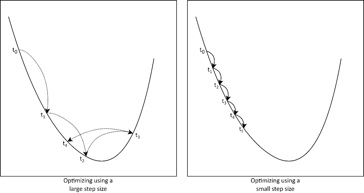
While a model is composed of parameters, the training algorithm has parameters of its own called hyperparameters. A hyperparameter is a controllable value that influences the training process or algorithm. For example, consider finding the minimum of a parabola function: we could start by guessing a value and then take small steps in the direction that minimizes the function output. The step size would have to be chosen well: if our steps are too small, it will take a prohibitively long time to find the minimum. If the step size is too large, we may overshoot and miss the minimum and then continue oscillating (jumping back and forth) around the minimum:

Figure 1.1 – Effect of using a step size that is too large (left) and too small (right)

In this example, the step size would be a hyperparameter of our minimization algorithm. The effect of the step size is illustrated in Figure 1.1.

Datasets

As explained previously, the machine learning model is trained using a dataset. Data is at the heart of the machine learning process, and data preparation is often the part of the process that takes up the most time.

Throughout this book, we’ll work with tabular datasets. Tabular datasets are very common in the real world and consist of rows and columns. Rows are often called samples, examples, or observations, and columns are usually called features, variables, or attributes.

Importantly, there is no restriction on the data type in a column. Features may be strings, numbers, Booleans, geospatial coordinates, or encoded formats such as audio, images, or video.

Datasets are also rarely perfectly defined. Data may be incomplete, noisy, incorrect, inconsistent, and contain various formats.

Therefore, data preparation and cleaning are essential parts of the machine learning process.

Data preparation concerns processing the data to make it suitable for machine learning and typically consists of the following steps:

1. Gathering and validation: Some datasets are initially too small or represent the problem poorly (the data is not representative of the actual data population it’s been sampled from). In these cases, the practitioner must collect more data, and validation must be done to ensure the data represents the problem.
2. Checking for systemic errors and bias: It is vital to check for and correct any systemic errors in the collection and validation process that may lead to bias in the dataset. In our sales example, a systemic collection error may be that data was only gathered from urban stores and excluded rural ones. A model trained on only urban store data will be biased in forecasting store sales, and we may expect poor performance when the model is used to predict sales for rural stores.
3. Cleaning the data: Any format or value range inconsistencies must be addressed. Any missing values also need to be handled in a way that does not introduce bias.
4. Feature engineering: Certain features may need to be transformed to ensure the machine learning model can learn from them, such as numerically encoding a sentence of words. Additionally, new features may need to be prepared from existing features to help the model detect patterns.
5. Normalizing and standardizing: The relative ranges of features must be normalized and standardized. Normalizing and standardizing ensure that no one feature has an outsized effect on the overall prediction.
6. Balancing the dataset: In cases where the dataset is imbalanced – that is, it contains many more examples of one class or prediction than another – the dataset needs to be balanced. Balancing is typically done by oversampling the minority examples to balance the dataset.

In Chapter 6, Solving Real-World Data Science Problems with LightGBM, we’ll go through the entire data preparation process to show how the preceding steps are applied practically.

Note

A good adage to remember is “garbage in, garbage out”. A model learns from any data given to it, including any flaws or biases contained in the data. When we train the model on garbage data, it results in a garbage model.

One final concept to understand regarding datasets is the training, validation, and test datasets. We split our datasets into these three subsets after the data preparation step is done:

• The training set is the most significant subset and typically consists of 60% to 80% of the data. This data is used to train the model.
• The validation set is separate from the training data and is used throughout the training process to evaluate the model. Having independent validation data ensures that the model is evaluated on data it has not seen before, also known as its generalization ability. Hyperparameter tuning, a process covered in detail in Chapter 5, LightGBM Parameter Optimization with Optuna, also uses the validation set.
• Finally, the test set is an optional hold-out set, similar to the validation set. It is used at the end of the process to evaluate the model’s performance on data that was not part of the training or tuning process.

Another use of the validation set is to monitor whether the model is overfitting the data. Let’s discuss overfitting in more detail.

Overfitting and generalization

To understand overfitting, we must first define what we mean by model generalization. As stated previously, generalization is the model’s ability to accurately predict data it has not seen before. Compared to training accuracy, generalization accuracy is more significant as an estimate of model performance as this indicates how our model will perform in production. Generalization comes in two forms, interpolation and extrapolation:

• Interpolation refers to the model’s ability to predict a value between two known data points – stated another way, to generalize within the training data range. For example, let’s say we train our model with monthly data from January to July. When interpolating, we would ask the model to make a prediction on a particular day in April, a date within our training range.
• Extrapolation, as you might infer, is the model’s ability to predict values outside of the range defined by our training data. A typical example of extrapolation is forecasting – that is, predicting the future. In our previous example, if we ask the model to make a prediction in December, we expect it to extrapolate from the training data.

Of the two types of generalization, extrapolation is much more challenging and may require a specific type of model to achieve. However, in both cases, a model can overfit the data, losing its ability to interpolate or extrapolate accurately.

Overfitting is a phenomenon where the model fits the training data too closely and loses its ability to generalize to unseen data. Instead of learning the underlying pattern in the data, the model has memorized the training data. More technically, the model fits the noise contained in the training data. The term noise stems from the concept of data containing signal and noise. Signal refers to the underlying pattern or information captured in the data we are trying to predict. In contrast, noise refers to random or irrelevant variations of data points that mask the signal.

For example, consider a dataset where we try to predict the rainfall for specific locations. The signal in the data would be the general trend of rainfall: rainfall increases in the winter or summer, or vice versa for other locations. The noise would be the slight variations in rainfall measurement for each month and location in our dataset.

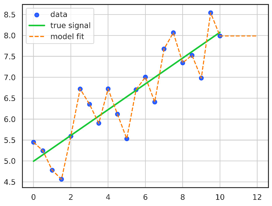
The following graph illustrates the phenomenon of overfitting:

Figure 1.2 – Graph showing overfitting. The model has overfitted and predicted the training data perfectly but has lost the ability to generalize to the actual signal

The preceding figure shows the difference between signal and noise: each data point was sampled from the actual signal. The data follows the general pattern of the signal, with slight, random variations. We can see how the model has overfitted the data: the model has fit the training data perfectly but at the cost of generalization. We can also see that if we use the model to interpolate by predicting a value for 4, we get a result much higher than the actual signal (6.72 versus 6.2). Also shown is the model’s failure to extrapolate: the prediction for 12 is much lower than a forecast of the signal (7.98 versus 8.6).

In reality, all real-world datasets contain noise. As data scientists, we aim to prepare the data to remove as much noise as possible, making the signal easier to detect. Data cleaning, normalization, feature selection, feature engineering, and regularization are techniques for removing noise from the data.

Since all real-world data contains noise, overfitting is impossible to eliminate. The following conditions may lead to overfitting:

• An overly complex model: A model that is too complex for the amount of data we have utilizes additional complexity to memorize the noise in the data, leading to overfitting
• Insufficient data: If we don’t have enough training data for the model we use, it’s similar to an overly complex model, which overfits the data
• Too many features: A dataset with too many features likely contains irrelevant (noisy) features that reduce the model’s generalization
• Overtraining: Training the model for too long allows it to memorize the noise in the dataset

As the validation set is a part of the training data that remains unseen by the model, we use the validation set to monitor for overfitting. We can recognize the point of overfitting by looking at the training and generalization errors over time. At the point of overfitting, the validation error increases. In contrast, the training error continues to improve: the model is fitting noise in the training data and losing its ability to generalize.

Techniques that prevent overfitting usually aim to address the conditions that lead to overfitting we discussed previously. Here are some strategies to avoid overfitting:

• Early stopping: We can stop training when we see the validation error beginning to increase.
• Simplifying the model: A less complex model with fewer parameters would be incapable of learning the noise in the training data, thereby generalizing better.
• Get more data: Either collecting more data or augmenting data is an effective method for preventing overfitting by giving the model a better chance to learn the signal in the data instead of the noise in a smaller dataset.
• Feature selection and dimensionality reduction: As some features might be irrelevant to the problem being solved, we can discard features we think are redundant or use techniques such as Principal Component Analysis to reduce the dimensionality (features).
• Adding regularization: Smaller parameter values typically lead to better generalization, depending on the model (a neural network is an example of such a model). Regularization adds a penalty term to the objective function to discourage large parameter values. By driving the parameters to smaller (or zero) values, they contribute less to the prediction, effectively simplifying the model.
• Ensemble methods: Combining the prediction from multiple, weaker models can lead to better generalization while also improving performance.

It’s important to note that overfitting and the techniques to prevent overfitting are specific to our model. Our goal should always be to minimize overfitting to ensure generalization to unseen data. Some strategies, such as regularization, might not work for specific models, while others might be more effective. There are also more bespoke strategies for models, an example of which we’ll see when we discuss overfitting in decision trees.

Supervised learning

The store sales example is an instance of supervised learning – we have a dataset consisting of features and are training the model to predict a target.

Supervised learning problems can be divided into two main types of problem categories: classification problems and regression problems.

Classification and regression

With a classification problem, the label that needs to be predicted by the model is categorical or defines a class. Some examples of classes are spam or not spam, cat or dog, and diabetic or not diabetic. These are examples of binary classifications: there are only two classes.

Multi-class classification is also possible; for example, email may be classified as Important, Promotional, Clutter, or Spam; images of clouds could be classified as Cirro, Cumulo, Strato, or Nimbo.

With regression problems, the goal is to predict a continuous, numerical value. Examples include predicting revenue, sales, temperature, house prices, and crowd size.

A big part of the art of machine learning is correctly defining or transcribing a problem as a classification or regression problem (or perhaps unsupervised or reinforcement). Later chapters will cover multiple end-to-end case studies of both types of problems.

Model performance metrics

Let’s briefly discuss how we measure our model’s performance. Model performance refers to the ability of a machine learning model to make accurate predictions or generate meaningful outputs based on the given inputs. An evaluation metric quantifies how well a model generalizes to new, unseen data. High model performance indicates that the model has learned the underlying patterns in the data effectively and can make accurate predictions on data it has not seen before. We can measure the model’s performance relative to the known targets when working with supervised learning problems (either classification or regression problems).

Importantly, how we measure the model’s performance on classification tasks and regression tasks differs. scikit-learn has many built-in metrics functions ready for use with either a classification or regression problem (https://scikit-learn.org/stable/modules/model_evaluation.html). Let’s review the most common of these.

Classification metrics can be defined in terms of positive and negative predictions made by the model. The following definitions can be used to calculate classification metrics:

• True positive (TP): A positive instance is correctly classified as positive
• True negative (TN): A negative instance is correctly classified as negative
• False positive (FP): A negative instance is incorrectly classified as positive
• False negative (FN): A positive instance is incorrectly classified as negative

Given these definitions, the most common classification metrics are as follows:

• Accuracy: Accuracy is the most straightforward classification metric. Accuracy is the number of correct predictions divided by the total number of predictions. However, accuracy is susceptible to an imbalance in the data. For example, suppose we have an email dataset with 8 examples of spam and 2 examples of non-spam, and our model predicts only spam. In that case, the model has an accuracy of 80%, even though it never correctly classified non-spam emails. Mathematically, we can define accuracy as follows:

  Accuracy =  TP + TN ______________  TP + FP + TN + FN 

• Precision: The precision score is one way of getting a more nuanced understanding of the classification performance. Precision is the ratio between the true positive prediction (correctly predicted) and all positive predictions (true positive and false positive). In other words, the precision score indicates how precise the model is in predicting positives. In our spam emails example, a model predicting only spam is not very precise (as it classifies all non-spam emails as spam) and has a lower precision score. The following formula can be used to calculate precision:

  Precision =  TP _ TP + FP 

• Recall: The recall score is the counterpoint to the precision score. The recall score measures how effectively the model finds (or recalls) all true positive cases. The recall is calculated as the ratio between true positive predictions and all positive instances (true positive and false negative). In our spam example, a model predicting only spam has perfect recall (it can find all the spam). We can calculate recall like so:

  Recall =  TP _ TP + FN 

• F1 score: Finally, we have the F1 score. The F1 score is calculated as the harmonic mean between precision and recall. The F1 score balances precision and recall, giving us a singular value that summarizes the classifier’s performance. The following formula can be used to calculate the F1 score:

  F 1 =  2 × Precision × Recall  _______________  Precision + Recall  =  2 × TP _____________  2 × TP + FP + FN 

The preceding classification metrics are the most common, but there are many more. Even though the F1 score is commonly used in classification problems (as it summarizes precision and recall), choosing the best metric is specific to the problem you are solving. Often, it might be the case that a specific metric is required, but other times, you must choose based on experience and your understanding of the data. We will look at examples of different metrics later in this book.

The following are common regression metrics:

• Mean squared error (MSE): The MSE is calculated as the average of the squared differences between predicted and actual values. The MSE is commonly used because of one crucial mathematical property: the MSE is differentiable and is therefore appropriate for use with gradient-based learning methods. However, since the difference is squared, the MSE penalizes large errors more heavily than small errors, which may or may not be appropriate to the problem being solved.
• Mean absolute error (MAE): Instead of squaring the differences, the MAE is calculated as the average of the absolute differences between predicted and actual values. By avoiding the square of errors, the MAE is more robust against the magnitude of errors and less sensitive to outliers than the MSE. However, the MAE is not differentiable and, therefore, can’t be used with gradient-based learning methods.

As with the classification metrics, choosing the most appropriate regression metric is specific to the problem you are trying to solve.

Metrics versus objectives

We defined training a model as finding the most appropriate parameters to minimize an objective function. It’s important to note that the objective function and metrics used for a specific problem may differ. A good example is decision trees, where a measure of impurity (entropy) is used as the objective function when building a tree. However, we still calculate the metrics explained previously to determine the tree’s performance on the data.

With our understanding of basic metrics in place, we can conclude our introduction to machine learning concepts. Now, let’s review the terms and concepts we’ve discussed using an example.

A modeling example

Consider the following data of sales by month, in thousands:

Table 1.1 – Sample sales data, by month, in thousands

This problem is straightforward: there is only one feature, the month, and the target is the number of sales. Therefore, this is an example of a supervised regression problem.

Note

You might have noticed that this is an example of a time series problem: time is the primary variable. Time series can also be predicted using more advanced time series-specific algorithms such as ANOVA, but we’ll use a simple algorithm for illustration purposes in this section.

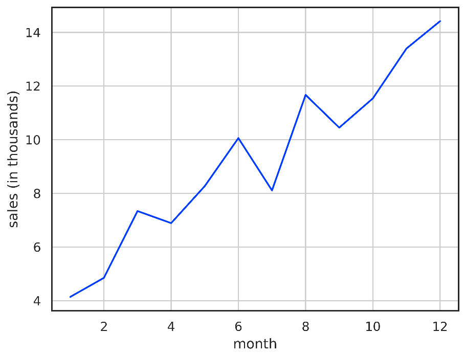
We can plot our data as a graph of sales per month to understand it better:

Figure 1.3 – Graph showing store sales by month

Here, we’re using a straight-line model, also known as simple linear regression, to model our sales data. The definition of a straight line is given by the following formula:

y = mx + c

Here, m is the line’s slope and c is the Y-intercept. In machine learning, the straight line is the model, and m and c are the model parameters.

To find the best parameters, we must measure how well our model fits the data for a particular set of parameters – that is, the error in our outputs. We will use the MAE as our metric:

MAE =  ∑ i=1 n  | ˆ y  − y| _ n 

Here,  ˆ y  is the predicted output, y is the actual output, and n is the number of predictions. We calculate the MAE by making a prediction for each of our inputs and then calculating the MAE based on the formula.

Fitting the model

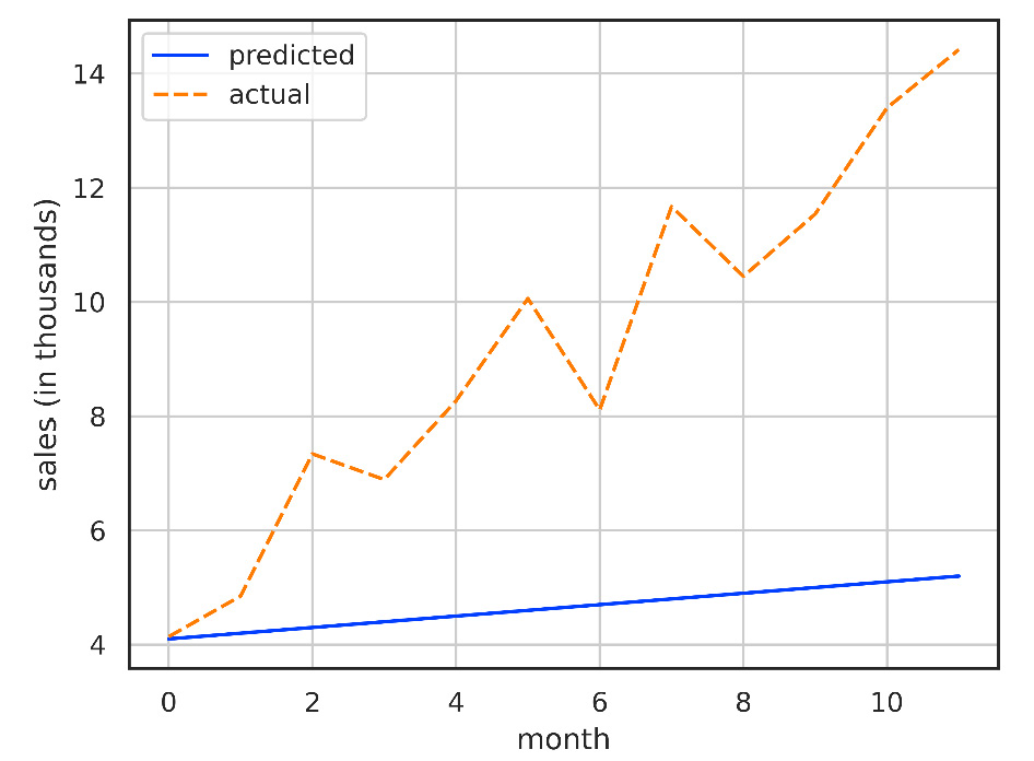
Now, let’s fit our linear model to our data. Our process for fitting the line is iterative, and we start this process by guessing values for m and c and then iterating from there. For example, let’s consider m = 0.1, c = 4:

Figure 1.4 – Graph showing the prediction of a linear model with m = 0.1 and c = 4

With these parameters, we achieve an error of 4,610.

Our guess is far too low, but that’s okay; we can now update the parameters to attempt to improve the error. In reality, updating the model parameters is done algorithmically using a training algorithm such as gradient descent. We’ll discuss gradient descent in Chapter 2, Ensemble Learning – Bagging and Boosting.

In this example, we’ll use our understanding of straight lines and intuition to update the parameters for each iteration manually. Our line is too shallow, and the intercept is too low; therefore, we must increase both values. We can control the updates we make each iteration by choosing a step size. We must update the m and c values with each iteration by adding the step size. The results, for a step size of 0.1, is shown in Table 1.2.

Table 1.2 – Step wise guessing of the slope (m) and y-intercept (c) for a straight line to fit our data. The quality of fit is measured using the MAE

In our example, the step size is a hyperparameter of our training process.

We end up with an error of 1.83, which means, on average, our predictions are wrong by less than 2,000.

Now, let’s see how we can solve this problem using scikit-learn.

Linear regression with scikit-learn

Instead of manually modeling, we can use scikit-learn to build a linear regression model. As this is our first example, we’ll walk through the code line by line and explain what’s happening.

To start with, we must import the Python tools we are going to use:

import numpy as np
import pandas as pd
from matplotlib import pyplot as plt
import seaborn as sns
from sklearn.linear_model import LinearRegression
from sklearn.metrics import mean_absolute_error

There are three sets of imports: we import numpy and pandas first. Importing NumPy and pandas is a widely used way to start all your data science notebooks. Also, note the short names np and pd, which are the standard conventions when working with numpy and pandas.

Next, we import a few standard plotting libraries we will use to plot some graphs: pyplot from matplotlib and seaborn. Matplotlib is a widely used plotting library that we access via the pyplot python interface. Seaborn is another visualization tool built on top of Matplotlib, which makes it easier to draw professional-looking graphs.

Finally, we get to our scikit-learn imports. In Python code, the scikit-learn library is called sklearn. From its linear_model package, we import LinearRegression. scikit-learn implements a wide variety of predefined metrics, and here, we will be using mean_absolute_error.

Now, we are ready to set up our data:

months = np.array([ 1,  2,  3,  4,  5,  6,  7,  8,  9, 10, 11, 12])
sales = np.array([4.14,  4.85,  7.34,  6.89,  8.27, 10.06,  8.11, 11.67, 10.45, 11.54, 13.4 , 14.42])
df = pd.DataFrame({"month": months, "sales": sales})

Here, we define a new numpy array for the months and the corresponding sales, and to make them easier to work with, we gather both arrays into a new pandas DataFrame.

With the data in place, we get to the interesting part of the code: modeling using scikit-learn. The code is straightforward:

model = LinearRegression()
model = model.fit(df[["month"]], df[["sales"]])

First, we create our model by constructing an instance of LinearRegression. We then fit our model using model.fit and passing in the month and sales data from our DataFrame. These two lines are all that’s required to fit a model, and as we’ll see in later chapters, even complicated models use the same recipe to instantiate and train a model.

We can now calculate our MAE by creating predictions for our data and passing the predictions and actual targets to the metric function:

predicted_sales = model.predict(df[["month"]])
mean_absolute_error(predicted_sales, df[["sales"]])

We get an error of 0.74, which is slightly lower than our guesswork. We can also examine the model’s coefficient and intercept (m and c from earlier):

print(f"Gradient: ${model.coef_}")
print(f"Intercept: ${model.intercept_}")

scikit-learn has fitted a model with a coefficient of 0.85 and an intercept of 3.68. We were in the right neighborhood with our guesses, but it might have taken us some time to get to the optimal values.

That concludes our introduction to scikit-learn and the basics of modeling and machine learning. In our toy example, we did not split our data into separate datasets, optimize our model’s hyperparameters, or apply any techniques to ensure our model does not overfit. In the next section, we’ll look at classification and regression examples, where we’ll apply these and other best practices.