-
Book Overview & Buying
-
Table Of Contents

The Data Science Workshop - Second Edition
By :
The Data Science Workshop
By:
Overview of this book
Where there’s data, there’s insight. With so much data being generated, there is immense scope to extract meaningful information that’ll boost business productivity and profitability. By learning to convert raw data into game-changing insights, you’ll open new career paths and opportunities.
The Data Science Workshop begins by introducing different types of projects and showing you how to incorporate machine learning algorithms in them. You’ll learn to select a relevant metric and even assess the performance of your model. To tune the hyperparameters of an algorithm and improve its accuracy, you’ll get hands-on with approaches such as grid search and random search.
Next, you’ll learn dimensionality reduction techniques to easily handle many variables at once, before exploring how to use model ensembling techniques and create new features to enhance model performance. In a bid to help you automatically create new features that improve your model, the book demonstrates how to use the automated feature engineering tool. You’ll also understand how to use the orchestration and scheduling workflow to deploy machine learning models in batch.
By the end of this book, you’ll have the skills to start working on data science projects confidently. By the end of this book, you’ll have the skills to start working on data science projects confidently.
Table of Contents (16 chapters)
Preface

1. Introduction to Data Science in Python
 Free Chapter
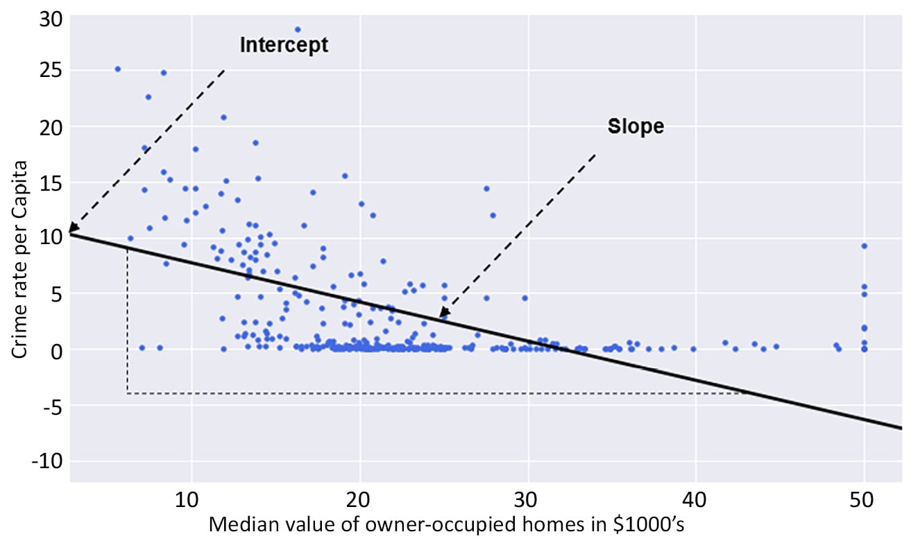
2. Regression
3. Binary Classification
4. Multiclass Classification with RandomForest
5. Performing Your First Cluster Analysis
6. How to Assess Performance
7. The Generalization of Machine Learning Models
8. Hyperparameter Tuning
9. Interpreting a Machine Learning Model
10. Analyzing a Dataset
11. Data Preparation
12. Feature Engineering
13. Imbalanced Datasets
14. Dimensionality Reduction