

Moving average and exponential smoothing
Possibly the simplest form of forecasting is the moving average. Often, a moving average is used as a smoothing technique to find a straighter line through data with a lot of variation. Each data point is adjusted to the value of the average of n surrounding data points, with n being referred to as the window size. With a window size of 10, for example, we would adjust a data point to be the average of the 5 values before and the 5 values after. In a forecasting setting, the future values are calculated as the average of the n previous values, so again, with a window size of 10, this means the average of the 10 previous values.
The balancing act with a moving average is that you want a large window size in order to smooth out the noise and capture the actual trend, but with a larger window size, your forecasts are going to lag the trend significantly as you reach back further and further to calculate the average. The idea behind exponential smoothing is to apply exponentially decreasing weights to the values being averaged over time, giving recent values more weight and older values less. This allows the forecast to be more reactive to changes, while still ignoring a good deal of noise.
As you can see in the following plot of simulated data, the moving average line exhibits much rougher behavior than the exponential smoothing line, but both lines still adjust to trend changes at the same time:
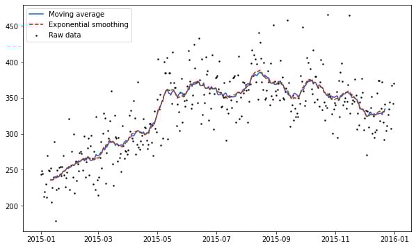
Figure 1.2 – Moving average versus exponential smoothing
Exponential smoothing originated in the 1950s with simple exponential smoothing, which does not allow for a trend or seasonality. Charles Holt advanced the technique in 1957 to allow for a trend with what he called double exponential smoothing; and in collaboration with Peter Winters, Holt added seasonality support in 1960, in what is commonly called Holt-Winters exponential smoothing.
The downside to these methods of forecasting is that they can be slow to adjust to new trends and so forecasted values lag behind reality—they do not hold up well to longer forecasting timeframes, and there are many hyperparameters to tune, which can be a difficult and very time-consuming process.