Visualizing data

A new connection to a data source is an invitation to explore and discover! At times, you may come to the data with very well-defined questions and a strong sense of what you expect to find. Other times, you will come to the data with general questions and very little idea of what you will find. The visual analytics capabilities of Tableau empower you to rapidly and iteratively explore the data, ask new questions, and make new discoveries.

The following visualization examples cover a few of the most foundational visualization types. As you work through the examples, keep in mind that the goal is not simply to learn how to create a specific chart. Rather, the examples are designed to help you think through the process of asking questions of the data and getting answers through iterations of visualization. Tableau is designed to make that process intuitive, rapid, and transparent.

Bar charts

Bar charts visually represent data in a way that makes the comparison of values across different categories easy. The length of the bar is the primary means by which you will visually understand the data. You may also incorporate color, size, stacking, and order to communicate additional attributes and values.

Creating bar charts in Tableau is very easy. Simply drag and drop the measure you want to see onto either the Rows or Columns shelf and the dimension that defines the categories onto the opposing Rows or Columns shelf.

As an analyst for Superstore, you are ready to begin a discovery process focused on sales (especially the dollar value of sales). As you follow the examples, work your way through the sheets in the Chapter 01 Starter workbook. The Chapter 01 Complete workbook contains the complete examples so that you can compare your results at any time:

1. Click on the Sales by Department tab to view that sheet.
2. Drag and drop the Sales field from Measures in the Data pane onto the Columns shelf. You now have a bar chart with a single bar representing the sum of sales for all of the data in the data source.
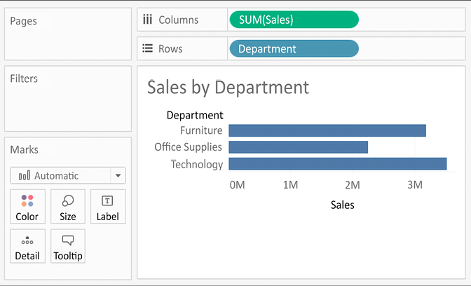
3. Drag and drop the Department field from Dimensions in the Data pane to the Rows shelf. This slices the data to give you three bars, each having a length that corresponds to the sum of sales for each department:

Figure 1.11: The view Sales by Department should look like this when you have completed the preceding steps

You now have a horizontal bar chart. This makes comparing the sales between the departments easy. The type drop-down menu on the Marks card is set to Automatic and indicates that Tableau has determined that bars are the best visualization given the fields you have placed in the view. As a dimension, Department slices the data. Being discrete, it defines row headers for each department in the data. As a measure, the Sales field is aggregated. Being continuous, it defines an axis. The mark type of bar causes individual bars for each department to be drawn from 0 to the value of the sum of sales for that department.

Tableau draws different marks in different ways; for example, bars are drawn from 0 (or the end of the previous bar, if stacked) along the axis. Circles and other shapes are drawn at locations defined by the value(s) of the field that is defining the axis. Take a moment to experiment with selecting different mark types from the drop-down menu on the Marks card. A solid grasp of how Tableau draws different mark types will help you to master the tool.

Iterations of bar charts for deeper analysis

Using the preceding bar chart, you can easily see that the Technology department has more total sales than either the Furniture or Office Supplies departments. What if you want to further understand sales amounts for departments across various regions? Follow these two steps:

1. Navigate to the Bar Chart (two levels) sheet, where you will find an initial view that is identical to the one you created earlier.
2. Drag the Region field from Dimensions in the Data pane to the Rows shelf and drop it to the left of the Department field already in view.

You should now have a view that looks like this:

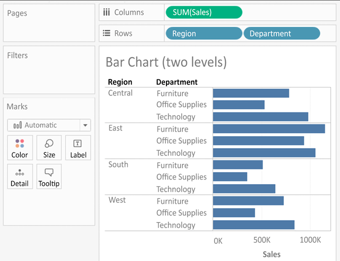
Figure 1.12: The view, Bar Chart (two levels), should look like this when you have completed the preceding steps

You still have a horizontal bar chart, but now you’ve introduced Region as another dimension, which changes the level of detail in the view and further slices the aggregate of the sum of sales. By placing Region before Department, you can easily compare the sales of each department within a given region.

Now you are starting to make some discoveries. For example, the Technology department has the most sales in every region, except in the East, where Furniture had higher sales. Office Supplies has never had the highest sales in any region.

Consider an alternate view, using the same fields arranged differently:

1. Navigate to the Bar Chart (stacked) sheet, where you will find a view that is identical to the original bar chart.
2. Drag the Region field from the Rows shelf and drop it onto the Color shelf:

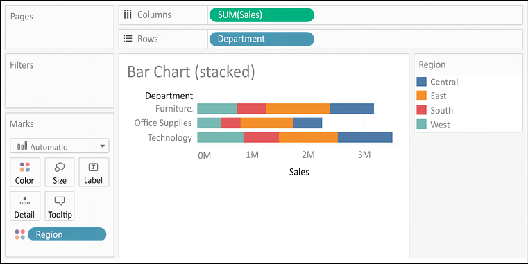
Figure 1.13: The Bar Chart (stacked) view should look like this

Instead of a side-by-side bar chart, you now have a stacked bar chart. Each segment of the bar is color-coded by the Region field. Additionally, a color legend has been added to the workspace. You haven’t changed the level of detail in the view, so sales are still summed for every combination of Region and Department.

Consider how the view level of detail changes based on the fields used in the view:

• If Department is the only field used as a dimension, you will have a view at the department level of detail, and all measures in the view will be aggregated per department.
• If Region is the only field used as a dimension, you will have a view at the region level of detail, and all measures in the view will be aggregated per region.
• If you use both Department and Region as dimensions in the view, you will have a view at the level of department and region. All measures will be aggregated per unique combination of department and region, and there will be one mark for each combination of department and region.

Stacked bars can be useful when you want to understand part-to-whole relationships. It is now easier to see what portion of the total sales of each department is made in each region. However, it is very difficult to compare sales for most of the regions across departments. For example, can you easily tell which department had the highest sales in the East region? It is difficult because, with the exception of the West region, every segment of the bar has a different starting point.

Now take some time to experiment with the bar chart to see what variations you can create:

1. Navigate to the Bar Chart (experimentation) sheet.
2. Try dragging the Region field from Color to the other various shelves on the Marks card, such as Size, Label, and Detail. Observe that in each case the bars remain stacked but are redrawn based on the visual encoding defined by the Region field.
3. Use the Swap button on the toolbar to swap fields on Rows and Columns. This allows you to very easily change from a horizontal bar chart to a vertical bar chart (and vice versa):

Figure 1.14: Swap Rows and Columns button

4. Drag and drop Sales from the Measures section of the Data pane on top of the Region field on the Marks card to replace it. Drag the Sales field to Color if necessary and notice how the color legend is a gradient for the continuous field.
5. Experiment further by dragging and dropping other fields onto various shelves. Note the behavior of Tableau for each action you take.
6. From the File menu, select Save.

As you continue to explore various iterations, you’ll gain confidence with the flexibility available to visualize your data.

Line charts

Line charts connect related marks in a visualization to show movement or a relationship between those connected marks. The position of the marks and the lines that connect them are the primary means of communicating the data. Additionally, you can use size and color to communicate additional information.

The most common kind of line chart is a time series. A time series shows the movement of values over time. Creating one in Tableau requires only a date and a measure.

Continue your analysis of Superstore sales using the Chapter 01 Starter workbook you just saved:

1. Navigate to the Sales over time sheet.
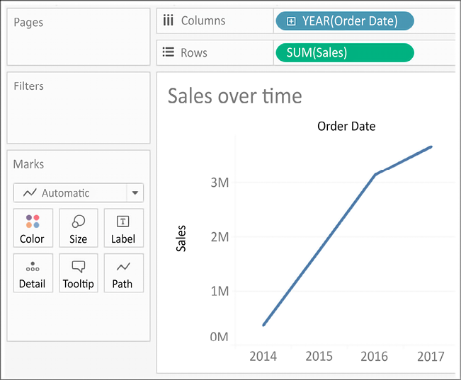
2. Drag the Sales field from Measures to Rows. This gives you a single, vertical bar representing the sum of all sales in the data source.
3. To turn this into a time series, you must introduce a date. Drag the Order Date field from Dimensions in the Data pane on the left and drop it into Columns. Tableau has a built-in date hierarchy, and the default level of Year has given you a line chart connecting four years. Notice that you can clearly see an increase in sales year after year:

Figure 1.15: An interim step in creating the final line chart; this shows the sum of sales by year

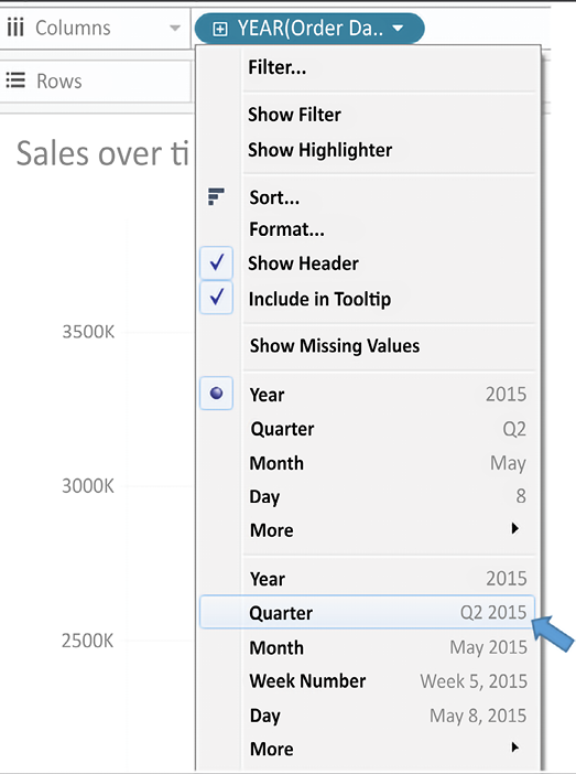
4. Use the drop-down menu on the YEAR(Order Date) field on Columns (or right-click on the field) and switch the date field to use Quarter. You may notice that Quarter is listed twice in the drop-down menu. We’ll explore the various options for date parts, values, and hierarchies in the Visualizing dates and times section of Chapter 3, Moving Beyond Basic Visualizations. For now, select the second option:

Figure 1.16: Select the second Quarter option in the drop-down menu.

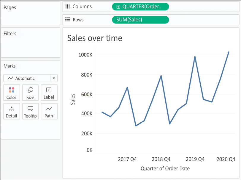
5. Notice that the cyclical pattern is quite evident when looking at sales by quarter:

Figure 1.17: Your final view shows sales over each quarter for the last several years

Let’s consider some variations of line charts that allow you to ask and answer even deeper questions.

Iterations of line charts for deeper analysis

Right now, you are looking at the overall sales over time. Let’s do some analysis at a slightly deeper level:

1. Navigate to the Sales over time (overlapping lines) sheet, where you will find a view that is identical to the one you just created.
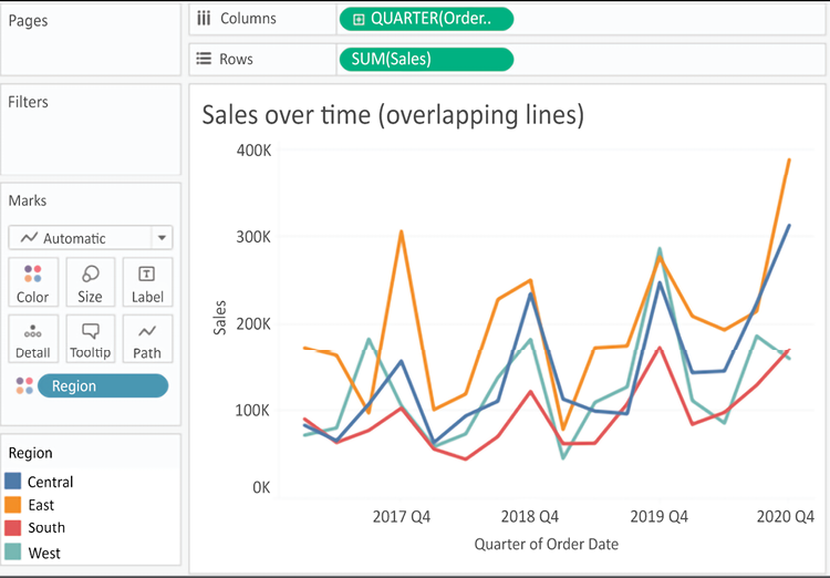
2. Drag the Region field from Dimensions to Color. Now you have a line per region, with each line a different color, and a legend indicating which color is used for which region. As with the bars, adding a dimension to Color splits the marks. However, unlike the bars, where the segments were stacked, the lines are not stacked. Instead, the lines are drawn at the exact value for the sum of sales for each region and quarter. This allows easy and accurate comparison. It is interesting to note that the cyclical pattern can be observed for each region:

Figure 1.18: This line chart shows the sum of sales by quarter with different colored lines for each region

With only four regions, it’s relatively easy to keep the lines separate. But what about dimensions that have even more distinct values? Let’s consider that case in the following example:

1. Navigate to the Sales over time (multiple rows) sheet, where you will find a view that is identical to the one you just created.
2. Drag the Category field from Dimensions and drop it directly on top of the Region field currently on the Marks card. This replaces the Region field with Category. You now have 17 overlapping lines. Often, you’ll want to avoid more than two or three overlapping lines. But you might also consider using color or size to showcase an important line in the context of the others. Also, note that clicking on an item in the Color legend will highlight the associated line in the view. Highlighting is an effective way to pick out a single item and compare it to all the others.
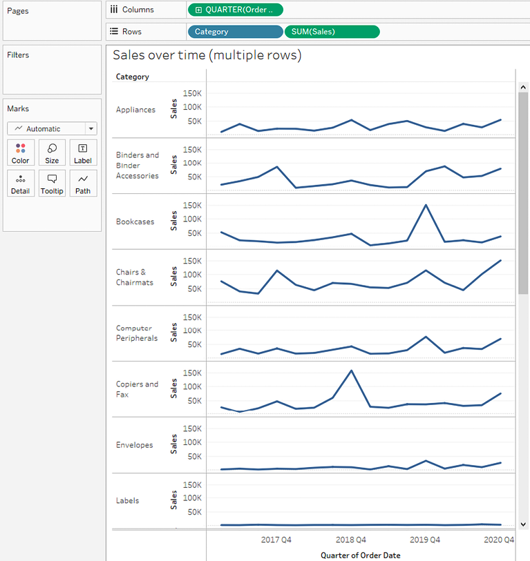
3. Drag the Category field from Color on the Marks card and drop it into Rows. You now have a line chart for each category. Now you have a way of comparing each product over time without an overwhelming overlap, and you can still compare trends and patterns over time. This is the start of a spark-lines visualization that will be developed more fully in Chapter 10, Advanced Visualizations:

Figure 1.19: Your final view should be a series of line charts for each category

The variations in lines for each Category allow you to notice variations in the trends, extremes, and rate of change.

Geographic visualizations

In Tableau, the built-in geographic database recognizes geographic roles for fields such as Country, State, City, Airport, Congressional District, or Zip Code. Even if your data does not contain latitude and longitude values, you can simply use geographic fields to plot locations on a map. If your data does contain latitude and longitude fields, you may use those instead of the generated values.

Tableau will automatically assign geographic roles to some fields based on a field name and a sampling of values in the data. You can assign or reassign geographic roles to any field by right-clicking on the field in the Data pane and using the Geographic Role option. This is also a good way to see what built-in geographic roles are available.

Geographic visualization is incredibly valuable when you need to understand where things happen and whether there are any spatial relationships within the data. Tableau offers several types of geographic visualization:

• Filled maps
• Symbol maps
• Density maps

Additionally, Tableau can read spatial files and geometries from some databases and render spatial objects, polygons, and more. We’ll take a look at these and other geospatial capabilities in Chapter 12, Exploring Mapping and Advanced Geospatial Features. For now, we’ll consider some foundational principles for geographic visualization.

Filled maps

Filled maps fill areas such as countries, states, or ZIP codes to show a location. The color that fills the area can be used to communicate measures such as average sales or population as well as dimensions such as region. These maps are also called choropleth maps.

Let’s say you want to understand sales for Superstore and see whether there are any patterns geographically.

You might take an approach like the following:

1. Navigate to the Sales by State sheet.
2. Double-click on the State field in the Data pane. Tableau automatically creates a geographic visualization using the Latitude (generated), Longitude (generated), and State fields.
3. Drag the Sales field from the Data pane and drop it on the Color shelf on the Marks card. Based on the fields and shelves you’ve used, Tableau has switched the automatic mark type to Map:

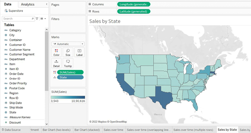
Figure 1.20: A filled map showing the sum of sales per state

The filled map fills each state with a single color to indicate the relative sum of sales for that state. The color legend, now visible in the view, gives the range of values and indicates that the state with the least sales had a total of 3,543 and the state with the most sales had a total of 1,090,616.

When you look at the number of marks displayed in the bottom status bar, you’ll see that it is 49. Careful examination reveals that the marks consist of the lower 48 states and Washington DC; Hawaii and Alaska are not shown. Tableau will only draw a geographic mark, such as a filled state, if it exists in the data and is not excluded by a filter.

Observe that the map does display Canada, Mexico, and other locations not included in the data. These are part of a background image retrieved from an online map service. The state marks are then drawn on top of the background image. We’ll look at how you can customize the map and even use other map services in the Mapping techniques section of Chapter 12, Exploring Mapping and Advanced Geospatial Features.

Filled maps can work well in interactive dashboards and have quite a bit of aesthetic value. However, certain kinds of analyses are very difficult with filled maps. Unlike other visualization types, where size can be used to communicate facets of the data, the size of a filled geographic region only relates to the geographic size and can make comparisons difficult. For example, which state has the highest sales? You might be tempted to say Texas or California because the larger size influences your perception, but would you have guessed Massachusetts? Some locations may be small enough that they won’t even show up compared to larger areas.

Use filled maps with caution and consider pairing them with other visualizations on dashboards for clear communication.

Symbol maps

With symbol maps, marks on the map are not drawn as filled regions; rather, marks are shapes or symbols placed at specific geographic locations. The size, color, and shape may also be used to encode additional dimensions and measures.

Continue your analysis of Superstore sales by following these steps:

1. Navigate to the Sales by Postal Code sheet.
2. Double-click on Postal Code under Dimensions. Tableau automatically adds Postal Code to Detail on the Marks card and Longitude (generated) and Latitude (generated) to Columns and Rows. The mark type is set to a circle by default, and a single circle is drawn for each postal code at the correct latitude and longitude.
3. Drag Sales from Measures to the Size shelf on the Marks card. This causes each circle to be sized according to the sum of sales for that postal code.
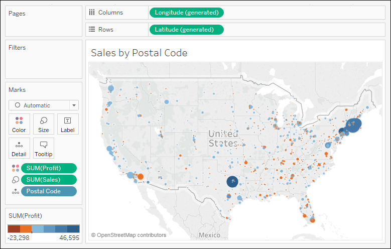
4. Drag Profit from Measures to the Color shelf on the Marks card. This encodes the mark color to correspond to the sum of profit. You can now see the geographic location of profit and sales at the same time. This is useful because you will see some locations with high sales and low profit, which may require some action.

The final view should look like this, after making some fine-tuned adjustments to the size and color:

Figure 1.21: A symbol map showing the sum of profit (encoded with color) and the sum of sales (encoded with size) per postal code

Sometimes, you’ll want to adjust the marks on a symbol map to make them more visible. Some options include the following:

• If the marks are overlapping, click on the Color shelf and set the transparency to somewhere between 50% and 75%. Additionally, add a dark border. This makes the marks stand out, and you can often better discern any overlapping marks.
• If marks are too small, click on the Size shelf and adjust the slider. You may also double-click on the Size legend and edit the details of how Tableau assigns size.
• If the marks are too faint, double-click on the Color legend and edit the details of how Tableau assigns color. This is especially useful when you are using a continuous field that defines a color gradient.

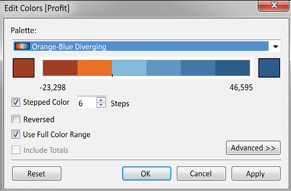
A combination of tweaking the size and using Stepped Color and Use Full Color Range, as shown here, produced the result for this example:

Figure 1.22: The Edit Colors dialog includes options for changing the number of steps, reversing, using the full color range, including totals, and advanced options for adjusting the range and center point

Unlike filled maps, symbol maps allow you to use size to visually encode aspects of the data. Symbol maps also allow greater precision. In fact, if you have latitude and longitude in your data, you can very precisely plot marks at a street address-level of detail. This type of visualization also allows you to map locations that do not have clearly defined boundaries.

Sometimes, when you manually select Map in the Marks card drop-down menu, you will get an error message indicating that filled maps are not supported at the level of detail in the view. In those cases, Tableau is rendering a geographic location that does not have built-in shapes.

Other than cases where filled maps are not possible, you will need to decide which type best meets your needs. We’ll also consider the possibility of combining filled maps and symbol maps in a single view in later chapters.

Density maps

Density maps show the spread and concentration of values within a geographic area. Instead of individual points or symbols, the marks blend together, showing greater intensity in areas with a high concentration. You can control the Color, Size, and Intensity.

Let’s say you want to understand the geographic concentration of orders. You might create a density map using the following steps:

1. Navigate to the Density of Orders sheet.
2. Double-click on the Postal Code field in the Data pane. Just as before, Tableau automatically creates a symbol map geographic visualization using the Latitude (generated), Longitude (generated), and State fields.
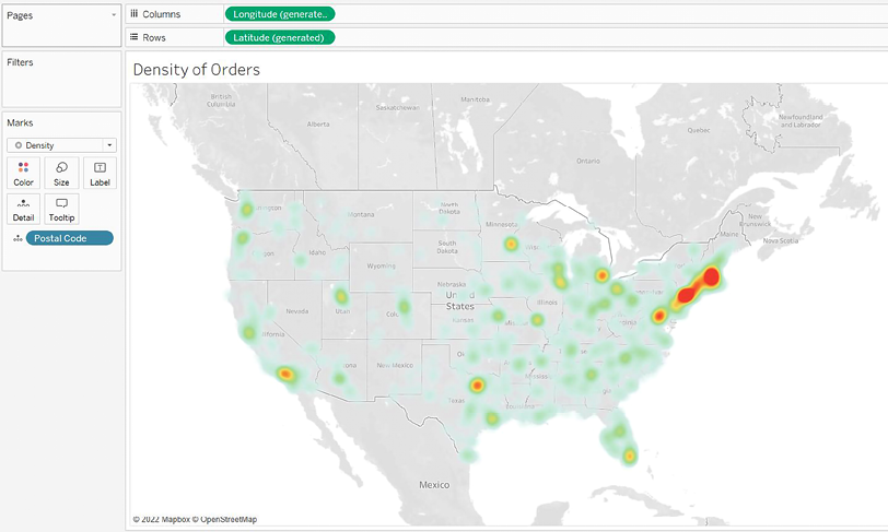
3. Using the drop-down menu on the Marks card, change the mark type to Density. The individual circles now blend together showing concentrations:

Figure 1.23: A density map showing concentration by postal code

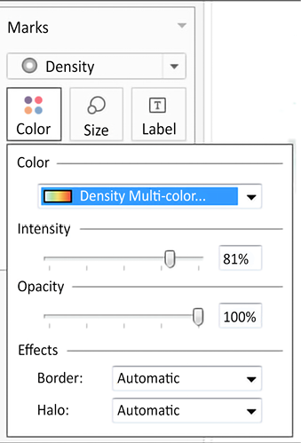
Try experimenting with the Color and Size options. Clicking on Color, for example, reveals some options specific to the Density mark type:

Figure 1.24: Options for adjusting the Color, Intensity, Opacity, and Effects for Density marks

Several color palettes are available that work well for density marks (the default ones work well with light color backgrounds, but there are others designed to work with dark color backgrounds). The Intensity slider allows you to determine how intensely the marks should be drawn based on concentrations. The Opacity slider lets you decide how transparent the marks should be.

This density map displays a high concentration of orders from the east coast. Sometimes, you’ll see patterns that merely reflect population density. In such cases, your analysis may not be particularly meaningful. In this case, the concentration on the east coast compared to the lack of density on the west coast is intriguing.

With an understanding of how to use Tableau to visualize your data, let’s turn our attention to a feature that generates some visualizations automatically, Show Me!