Up until this point, we have learned how to represent and preprocess text data. It’s time to make use of this knowledge and create the spam classifier. First, we put all the pieces together using a publicly available corpus. Before we proceed to the training of the classifier, we need to follow a series of typical steps that include the following:
- Getting the data
- Splitting it into a training and test set
- Preprocessing its content
- Extracting the features
Let’s examine each step one by one.
Getting the data
The SpamAssassin public mail corpus (https://spamassassin.apache.org/old/publiccorpus/) is a selection of email messages suitable for developing spam filtering systems. It offers two variants for the messages, either in plain text or HTML formatting. For simplicity, we will use only the first type in this exercise. Parsing HTML text requires special handling – for example, implementing your own regexps! The term coined to describe the opposite of spam emails is ham since the two words are related to meat products (spam refers to canned ham). The dataset contains various examples divided into different folders according to their complexity. This exercise uses the files within these two folders: spam_2 (https://github.com/PacktPublishing/Machine-Learning-Techniques-for-Text/tree/main/chapter-02/data/20050311_spam_2/spam_2) for spam and hard_ham (https://github.com/PacktPublishing/Machine-Learning-Techniques-for-Text/tree/main/chapter-02/data/20030228_hard_ham/hard_ham) for ham.
Creating the train and test sets
Initially, we read the messages for the two categories (ham and spam) and split them into training and testing groups. As a rule of thumb, we can choose a 75:25 (https://en.wikipedia.org/wiki/Pareto_principle) split between the two sets, attributing a more significant proportion to the training data. Note that other ratios might be preferable depending on the size of the dataset. Especially for massive corpora (with millions of labeled instances), we can create test sets with just 1% of the data, which is still a significant number. To clarify this process, we divide the code into the following steps:
- First, we load the ham and spam datasets using the
train_test_split method. This method controls the size of the training and test sets for each case and the samples that they include:import email
import glob
import numpy as np
from operator import is_not
from functools import partial
from sklearn.model_selection import train_test_split
# Load the path for each email file for both categories.
ham_files = train_test_split(glob.glob('./data/20030228_hard_ham/hard_ham/*'), random_state=123)
spam_files = train_test_split(glob.glob('./data/20050311_spam_2/spam_2/*'), random_state=123)
- Next, we read the content of each email and keep the ones without HTML formatting:
# Method for getting the content of an email.
def get_content(filepath):
    file = open(filepath, encoding='latin1')
    message = email.message_from_file(file)
    for msg_part in message.walk():
        # Keep only messages with text/plain content.
        if msg_part.get_content_type() == 'text/plain':
            return msg_part.get_payload()
# Get the training and testing data.
ham_train_data = [get_content(i) for i in ham_files[0]]
ham_test_data = [get_content(i) for i in ham_files[1]]
spam_train_data = [get_content(i) for i in spam_files[0]]
spam_test_data = [get_content(i) for i in spam_files[1]]
- For our analysis, we exclude emails with empty content. The
filter method with None as the first argument removes any element that includes an empty string. Then, the filtered output is used to construct a new list using list:# Keep emails with non-empty content.
ham_train_data = list(filter(None, ham_train_data))
ham_test_data = list(filter(None, ham_test_data))
spam_train_data = list(filter(None, spam_train_data))
spam_test_data = list(filter(None, spam_test_data))
- Now, let’s merge the spam and ham training sets into one (do the same for their test sets):
# Merge the train/test files for both categories.
train_data = np.concatenate((ham_train_data, spam_train_data))
test_data = np.concatenate((ham_test_data, spam_test_data))
- Finally, we assign a class label for each of the two categories (ham and spam) and merge them into common training and test sets:
# Assign a class for each email (ham = 0, spam = 1).
ham_train_class = [0]*len(ham_train_data)
ham_test_class = [0]*len(ham_test_data)
spam_train_class = [1]*len(spam_train_data)
spam_test_class = [1]*len(spam_test_data)
# Merge the train/test classes for both categories.
train_class = np.concatenate((ham_train_class, spam_train_class))
test_class = np.concatenate((ham_test_class, spam_test_class))
Notice that in step 1, we also pass random_state in the train_test_split method to make all subsequent results reproducible. Otherwise, the method performs a different data shuffling in each run and produces random splits for the sets.
In this section, we have learned how to read text data from a set of files and keep the information that makes sense for the problem under study. After this point, the datasets are suitable for the next processing phase.
Preprocessing the data
It’s about time to use the typical data preprocessing techniques that we learned earlier. These include tokenization, stop word removal, and lemmatization. Let’s examine the steps one by one:
- First, let’s tokenize the train or test data:
from nltk.stem import WordNetLemmatizer
from nltk.tokenize import word_tokenize
from sklearn.feature_extraction.text import ENGLISH_STOP_WORDS
# Tokenize the train/test data.
train_data = [word_tokenize(i) for i in train_data]
test_data = [word_tokenize(i) for i in test_data]
- Next, we remove the stop words by iterating over the
input examples:# Method for removing the stop words.
def remove_stop_words(input):
result = [i for i in input if i not in ENGLISH_STOP_WORDS]
return result
# Remove the stop words.
train_data = [remove_stop_words(i) for i in train_data]
test_data = [remove_stop_words(i) for i in test_data]
- Now, we create the lemmatizer and apply it to the words:
# Create the lemmatizer.
lemmatizer = WordNetLemmatizer()
# Method for lemmatizing the text.
def lemmatize_text(input):
    return [lemmatizer.lemmatize(i) for i in input]
# Lemmatize the text.
train_data = [lemmatize_text(i) for i in train_data]
test_data = [lemmatize_text(i) for i in test_data]
- Finally, we reconstruct the data in the two sets by joining the words separated by a space and return the concatenated string:
# Reconstruct the data.
train_data = [" ".join(i) for i in train_data]
test_data = [" ".join(i) for i in test_data]
As a result, we have at our disposal two Python lists, namely train_data and test_data, containing the initial text data in a processed form suitable for proceeding to the next phase.
Extracting the features
We continue with the extraction of the features of each sentence in the previously created datasets. This step uses tf-idf vectorization after training the vectorizer with the training data. There is a problem though, as the vocabulary in the training and test sets might differ. In this case, the vectorizer ignores unknown words, and depending on the mismatch level, we might get suboptimal representations for the test set. Hopefully, as more data is added to any corpus, the mismatch becomes smaller, so ignoring a few words has a negligible practical impact. An obvious question is – why not train the vectorizer with the whole corpus before the split? However, this engenders the risk of getting performance measures that are too optimistic later in the pipeline, as the model has seen the test data at some point. As a rule of thumb, always keep the test set separate and only use it to evaluate the model.
In the code that follows, we vectorize the data in both the training and test sets using tf-idf:
from sklearn.feature_extraction.text import TfidfVectorizer
# Create the vectorizer.
vectorizer = TfidfVectorizer()
# Fit with the train data.
vectorizer.fit(train_data)
# Transform the test/train data into features.
train_data_features = vectorizer.transform(train_data)
test_data_features = vectorizer.transform(test_data)
Now, the training and test sets are transformed from sequences of words to numerical vectors. From this point on, we can apply any sophisticated algorithm we wish, and guess what? This is what we are going to do in the following section!
Introducing the Support Vector Machines algorithm
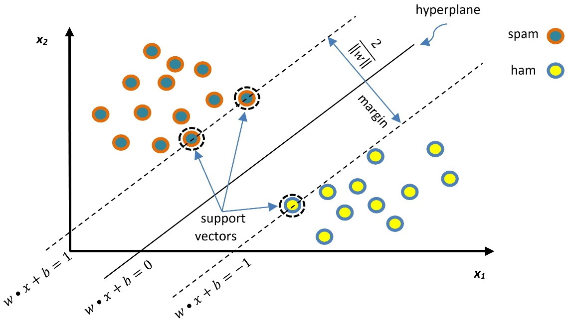
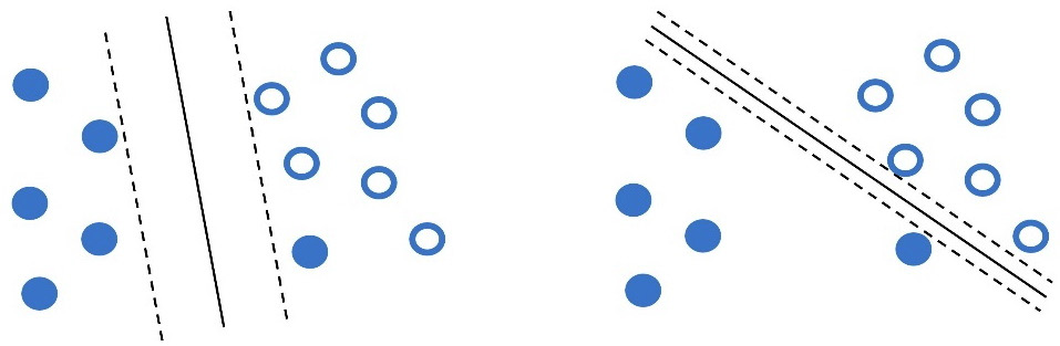
It’s about time that we train the first classification model. One of the most well-known supervised learning algorithms is the Support Vector Machines (SVM) algorithm. We could dedicate a whole book to demystifying this family of methods, so we will visit a few key elements in this section. First, recall from Chapter 1, Introducing Machine Learning for Text, that any ML algorithm creates decision boundaries to classify new data correctly. As we cannot sketch high-dimensional spaces, we will consider a two-dimensional example. Hopefully, this provides some of the intuition behind the algorithm.
Figure 2.9 shows the data points for the spam and ham instances along with two features, namely  and
and  :
:
Figure 2.9 – Classification of spam and ham emails using the SVM
The line in the middle separates the two classes and the dotted lines represent the borders of the margin. The SVM has a twofold aim to find the optimal separation line (a one-dimensional hyperplane) while maximizing the margin. Generally, for an n-dimensional space, the hyperplane has (n-1) dimensions. Let’s examine our space size in the code that follows:
print(train_data_features.shape)
>> (670, 28337)
Each of the 670 emails in the training set is represented by a feature vector with a size of 28337 (the number of unique words in the corpus). In this sparse vector, the non-zero values signify the tf-idf weights for the words. For the SVM, the feature vector is a point in a 28,337-dimensional space, and the problem is to find a 28,336-dimensional hyperplane to separate those points. One crucial consideration within the SVM is that not all the data points contribute equally to finding the optimal hyperplane, but mostly those close to the margin boundaries (depicted with a dotted circle in Figure 2.9). These are called support vectors, and if they are removed, the position of the dividing hyperplane alters. For this reason, we consider them the critical part of the dataset.
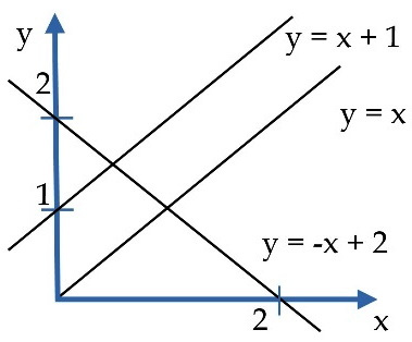
The general equation of a line in two-dimensional space is expressed with the formula  . Three examples are shown in Figure 2.10:
Figure 2.10 – Examples of line equations
In the same sense, the middle line in Figure 2.9 and the two margin boundaries have the following equations, respectively:
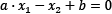 ,
, 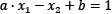 and
and 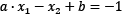
Defining the vectors  and
and  , we can rewrite the previous equations using the dot product that we encountered in the Calculating vector similarity section:
 ,
,  , and
, and 
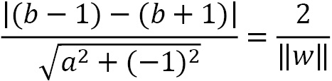
To find the best hyperplane, we need to estimate w and b, referred to as the weight and bias in ML terminology. Among the infinite number of lines that separate the two classes, we need to find the one that maximizes the margin, the distance between the closest data points of the two classes. In general, the distance between two parallel lines  and
and  is equal to the following:

So, the distance between the two margin boundaries is the following:
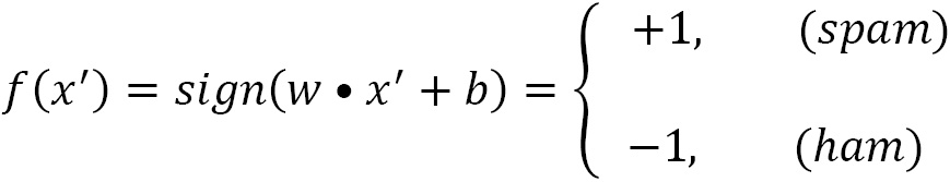
To maximize the previous equation, we need to minimize the denominator, namely the quantity  that represents the Euclidean norm of vector w. The technique for finding w and b is beyond the scope of this book, but we need to define and solve a function that penalizes any misclassified examples within the margin. After this point, we can classify a new example,
  , based on the following model (the sign function takes any number as input and returns +1 if it is positive or -1 if it is negative):
The example we are considering in Figure 2.9 represents an ideal situation. The data points are arranged in the two-dimensional space in such a way that makes them linearly separable. However, this is often not the case, and the SVM incorporates kernel functions to cope with nonlinear classification. Describing the mechanics of these functions further is beyond the scope of the current book. Notice that different kernel functions are available, and as in all ML problems, we have to experiment to find the most efficient option in any case. But before using the algorithm, we have to consider two important issues to understand the SVM algorithm better.
Adjusting the hyperparameters
Suppose two decision boundaries (straight lines) can separate the data in Figure 2.11.
Figure 2.11 – Two possible decision boundaries for the data points using the SVM
Which one of those boundaries do you think works better? The answer, as in most similar questions, is that it depends! For example, the line in the left plot has a higher classification error, as one opaque dot resides on the wrong side. On the other hand, the margin in the right plot (distance between the dotted lines) is small, and therefore the model lacks generalization. In most cases, we can tolerate a small number of misclassifications during SVM training in favor of a hyperplane with a significant margin. This technique is called soft margin classification and allows some samples to be on the wrong side of the margin.
The SVM algorithm permits the adjustment of the training accuracy versus generalization tradeoff using the hyperparameter C. A frequent point of confusion is that hyperparameters and model parameters are the same things, but this is not true. Hyperparameters are parameters whose values are used to control the learning process. On the other hand, model parameters update their value in every training iteration until we obtain a good classification model. We can direct the SVM to create the most efficient model for each problem by adjusting the hyperparameter C. The left plot of Figure 2.11 is related to a lower C value compared to the one on the right.
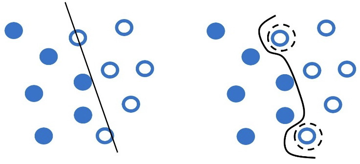
Let’s look at another dataset for which two possible decision boundaries exist (Figure 2.12). Which one seems to work better this time?
Figure 2.12 – Generalization (left) versus overfitting (right)
At first glance, the curved line in the plot on the right perfectly separates the data into two classes. But there is a problem. Getting too specific boundaries entails the risk of overfitting, where your model learns the training data perfectly but fails to classify a slightly different example correctly.
Consider the following real-world analogy of overfitting. Most of us have grown in a certain cultural context, trained (overfitted) to interpret social signals such as body posture, facial expressions, or voice tone in a certain way. As a result, when socializing with people of diverse backgrounds, we might fail to interpret similar social signals correctly (generalization).
Besides the hyperparameter C that can prevent overfitting, we can combine it with gamma, which defines how far the influence of a single training example reaches. In this way, the curvature of the decision boundary can also be affected by points that are pretty far from it. Low gamma values signify far reach of the influence, while high values cause the opposite effect. For example, in Figure 2.12 (right), the points inside a dotted circle have more weight, causing the line’s intense curvature around them. In this case, the hyperparameter gamma has a higher value than the left plot.
The takeaway here is that both C and gamma hyperparameters help us create more efficient models but identifying their best values demands experimentation. Equipped with the basic theoretical foundation, we are ready to incorporate the algorithm!
Putting the SVM into action
In the following Python code, we use a specific implementation of the SVM algorithm, the C-Support Vector Classification. By default, it uses the Radial Basis Function (RBF) kernel:
from sklearn import svm
# Create the classifier.
svm_classifier = svm.SVC(kernel="rbf", C=1.0, gamma=1.0, probability=True)
# Fit the classifier with the train data.
svm_classifier.fit(train_data_features.toarray(), train_class)
# Get the classification score of the train data.
svm_classifier.score(train_data_features.toarray(), train_class)
>> 0.9970149253731343
Now, use the test set:
# Get the classification score of the test data.
svm_classifier.score(test_data_features.toarray(), test_class)
>> 0.8755760368663594
Observe the classifier’s argument list, including the kernel and the two hyperparameters, gamma and C. Then, we evaluate its performance for both the training and test sets. We are primarily interested in the second result, as it quantifies the accuracy of our model on unseen data – essentially, how well it generalizes. On the other hand, the performance on the training set indicates how well our model has learned from the training data. In the first case, the accuracy is almost 100%, whereas, for unseen data, it is around 88%.
Equipped with the necessary understanding, you can rerun the preceding code and experiment with different values for the hyperparameters; typically, 0.1 < C < 100 and 0.0001 < gamma < 10. In the following section, we present another classification algorithm based on a fundamental theorem in ML.
Understanding Bayes’ theorem
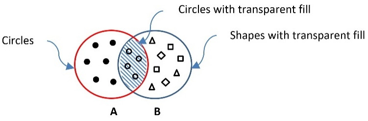
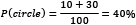
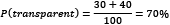
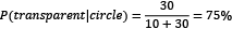
Imagine a pool of 100 shapes (including squares, triangles, circles, and rhombuses). These can have either an opaque or a transparent fill. If you pick a circle shape from the pool, what is the probability of it having a transparent fill? Looking at Figure 2.13, we are interested to know which shapes in set A (circles) are also members of set B (all transparent shapes):
Figure 2.13 – The intersection of the set with circles with the set of all transparent shapes
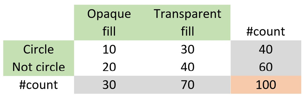
The intersection of the two sets is highlighted with the grid texture and mathematically written as A∩B or B∩A. Then, we construct Table 2.6, which helps us perform some interesting calculations:
Table 2.6 – The number of shapes by type and fill
First, notice that the total number of items in the table equals 100 (the number of shapes). We can then calculate the following quantities:
- The probability of getting a circle is
- The probability of getting a transparent fill is
- The probability of getting a transparent fill when the shape is a circle is
- The probability of getting a circle when the fill is transparent is
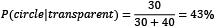
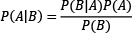
The symbol  signifies conditional probability. Based on these numbers, we can identify a relationship between the probabilities:

The previous equation suggests that if the probability P(transparent|circle) is unknown, we can use the others to calculate it. We can also generalize the equation as follows:

Exploring the different elements, we reach the famous formula known as Bayes’ theorem, which is fundamental in information theory and ML:
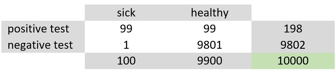
The exercise in Table 2.6 was just an example to introduce the fundamental reasoning behind the theorem; all quantities are available to calculate the corresponding probabilities. However, this is not the case in most practical problems, and this is where Bayes’ theorem comes in handy. For example, consider the following situation: you are concerned that you have a severe illness and decide to go to the hospital for a test. Sadly, the test is positive. According to your doctor, the test has 99% reliability; for 99 out of 100 sick people, the test is positive, and for 99 out of 100 healthy people, the test is negative. So, what is the probability of you having the disease? Most people logically answer 99%, but this is not true. The Bayesian reasoning tells us why.
We have a population of 10,000 people, and according to statistics, 1% (so, 100 people) of this population has the illness. Therefore, based on a 99% reliability, this is what we know:
- Of the 100 sick subjects, 99 times (99%), the test is positive, and 1 is negative (1% and therefore wrong).
- Of the 9,900 healthy subjects, 99 times (1%), the test is positive, and 9,801 is negative (99% and therefore correct).
As before, we construct Table 2.7, which helps us with the calculations:
Table 2.7 – The number of people by health condition and test outcome
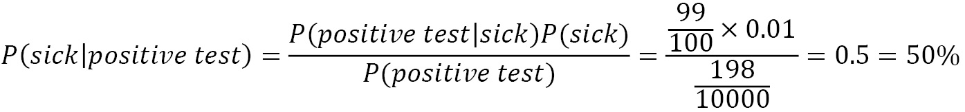
At first glance, the numbers suggest that there is a non-negligible likelihood that you are healthy and that the test is wrong (99/10000≈1%). Next, we are looking for the probability of being sick given a positive test. So, let’s see the following:
This percentage is much smaller than the 99% initially suggested by most people. What is the catch here? The probability P(sick) in the equation is not something we know exactly, as in the case of the shapes in the previous example. It’s merely our best estimate on the problem, which is called prior probability. The knowledge we have before delving into the problem is the hardest part of the equation to figure out.
Conversely, the probability P(sick|positive test) represents our knowledge after solving the problem, which is called posterior probability. If, for example, you retook the test and this showed to be positive, the previous posterior probability becomes your new prior one – the new posterior increases, which makes sense. Specifically, you did two tests, and both were positive.
Takeaway
Bayesian reasoning tells us how to update our prior beliefs in light of new evidence. As new evidence surfaces, your predictions become better and better.
Remember this discussion the next time you read an article on the internet about an illness! Of course, you always need to interpret the percentages in the proper context. But let’s return to the spam filtering problem and see how to apply the theorem in this case.
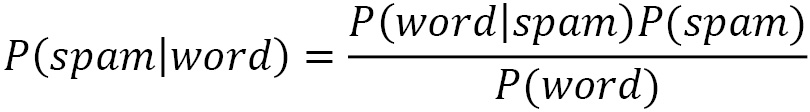
Introducing the Naïve Bayes algorithm
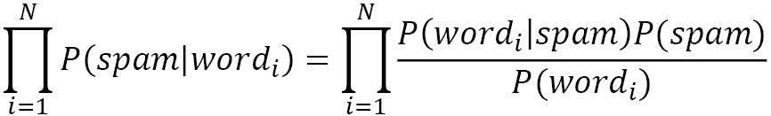
Naïve Bayes is a classification algorithm based on Bayes’ theorem. We already know that the features in the emails are the actual words, so we are interested in calculating each posterior probability P(spam|word) with the help of the following theorem:
where  .
.
Flipping a coin once gives a ½ probability of getting tails. The probability of getting tails two consecutive times is ¼, as P(tail first time)P(tail second time)=(½)(½)=¼. Thus, repeating the previous calculation for each word in the email (N words in total), we just need to multiply their individual probabilities:
As with the SVM, it is straightforward to incorporate Naïve Bayes using sklearn. In the following code, we use the algorithm’s MultinomialNB implementation to suit the discrete values (word counts) used as features better:
from sklearn import naive_bayes
# Create the classifier.
nb_classifier = naive_bayes.MultinomialNB(alpha=1.0)
# Fit the classifier with the train data.
nb_classifier.fit(train_data_features.toarray(), train_class)
# Get the classification score of the train data.
nb_classifier.score(train_data_features.toarray(), train_class)
>> 0.8641791044776119
Next, we incorporate the test set:
# Get the classification score of the test data.
nb_classifier.score(test_data_features.toarray(), test_class)
>> 0.8571428571428571
The outcome suggests that the performance of this classifier is inferior. Also, notice the result on the actual training set, which is low and very close to the performance on the test set. These numbers are another indication that the created model is not working very well.
Clarifying important key points
Before concluding this section, we must clarify some points concerning the Naïve Bayes algorithm. First of all, it assumes that a particular feature in the data is unrelated to the presence of any other feature. In our case, the assumption is that the words in an email are conditionally independent of each other, given that the type of the email is known (either spam or ham). For example, encountering the word deep does not suggest the presence or the absence of the word learning in the same email. Of course, we know that this is not the case, and many words tend to appear in groups (remember the discussion about n-grams). Most of the time, the assumption of independence of words is false and naive, and this is what the algorithm’s name stems from. In reality, of course, the assumption of independence allows us to solve many practical problems.
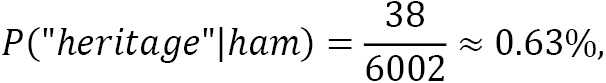
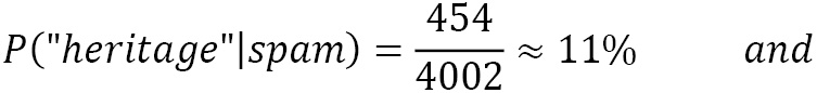
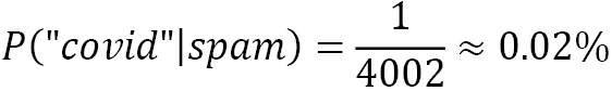
Another issue is when a word appears in the ham emails but is not present in the spam ones (say, covid). Then, according to the algorithm, its conditional probability is zero, P(“covid”|spam) = 0, which is rather inconvenient since we are going to multiply it with the other probabilities (making the outcome equal to zero). This situation is often known as the zero-frequency problem. The solution is to apply smoothing techniques such as Laplace smoothing, where the word count starts at 1 instead of 0.
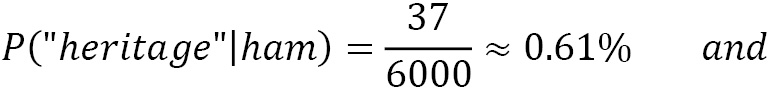
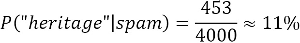
Let’s see an example of this problem. In a corpus of 10,000 emails, 6,000 are ham and 4,000 are spam. The word heritage appears in 37 emails of the first category and 453 of the second one. Its conditional probabilities are the following:
Moreover:
For an email that contains both words (heritage and covid), we need to multiply their individual probabilities (the symbol “…” signifies the other factors in the multiplication):
To overcome this problem, we apply Laplace smoothing, adding 1 in the numerator and 2 in the denominator. As a result, the smoothed probabilities now become the following:
Notice that Laplace smoothing is a hyperparameter that you can specify before running the classification algorithm. For example, in the Python code used in the previous section, we constructed the MultinomialNB classifier using the alpha=1.0 smoothing parameter in the argument list.
This section incorporated two well-known classification algorithms, the SVM and Naïve Bayes, and implemented two versions of a spam detector. We saw how to acquire and prepare the text data for training models, and we got a better insight into the trade-offs while adjusting the hyperparameters of the classifiers. Finally, this section provided some preliminary performance scores, but we still lack adequate knowledge to assess the two models. This discussion is the topic of the next section.


 Free Chapter