The Machine Learning Process

The machine learning process is a sequence of activities performed to deploy a successful model for prediction. A few steps here are iterative and can be repeated based on the outcomes of the previous and the following steps. To train a good model, we must clean our data and understand it well from the business perspective. Using our understanding, we can generate appropriate features. The performance of the model depends on the goodness of the features.

A sample model building process follows these steps:

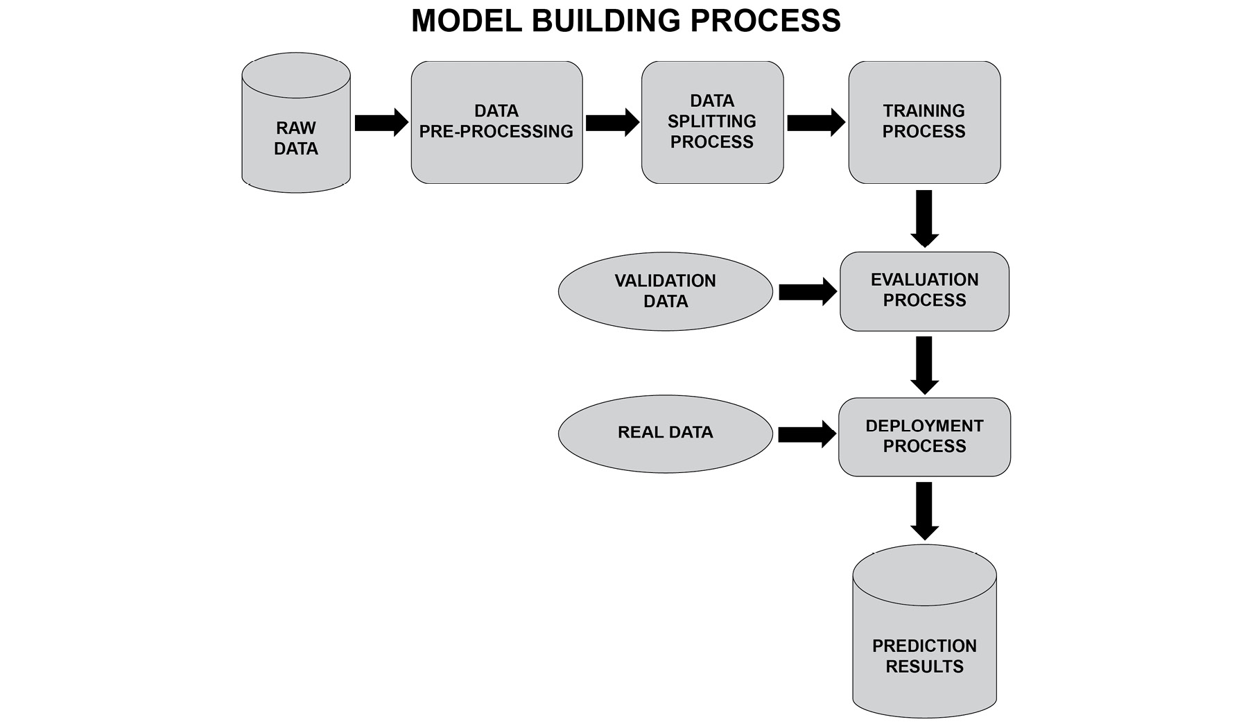
Figure 1.1: The model building process

The model building process consists of obtaining the right data, processing it to derive features, and then choosing the right model. Based on the type of output to be predicted, we need to choose a model. For example, if the output is categorical, a decision tree can be chosen; if the output is numerical, a neural network can be chosen. However, decision trees also can be used for regression and neural networks can be used for classification. Choosing the right data means using data related to the output of our problem. For example, if we are predicting the value of a house, then information such as the location and size are all data that is highly correlated with the predicted value, hence it is of high value. Gathering and deriving good features can make a huge difference.

Raw Data

The raw data refers to the unprocessed data that is relevant for the machine learning problem. For instance, if the problem statement is to predict the value of stocks, then the data constituting the characteristics of a stock and the company profile data may be relevant to the prediction of the stock value; therefore, this data is known as the raw data.

Data Pre-Processing

The pre-processing step involves:

1. Data cleaning
2. Feature selection
3. Computing new features

The data cleaning step refers to activities such as handling missing values in the data, handling incorrect values, and so on. During the feature selection process, features that correlate with the output or otherwise are termed important are selected for the purpose of modeling. Additional meaningful features that have high correlation with the output to be predicted can also be derived; this helps to improve the model performance.

The Data Splitting Process

The data can be split into an 80%-20% ratio, where 80% of the data is used to train the model and 20% of the data is used to test the model. The accuracy of the model on the test data is used as an indicator of the performance of the model.

Therefore, data is split as follows:

• Training data [80% of the data]: When we split our training data, we must ensure that 80% of the data has sufficient samples for the different scenarios we want to predict. For instance, if we are predicting whether it will rain or not, we usually want the training data to contain 40-60% of rows that represent will rain scenarios and 40-60% of rows that represent will not rain scenario.
• Testing data [20% of the data]: 20% of the data reserved for testing purposes must have a sample for the different cases/classes we are predicting for.
• Validation data [new data]: The validation data is any unseen data that is passed to the model for prediction. The measure of error on the validation data is also an indicator of the performance of the model.

The Training Process

The training phase involves the following:

1. Selecting a model
2. Training the model
3. Measuring the performance
4. Tuning the model

A machine learning model is selected for the purpose of training. The performance of the model is measured in the form of precision, recall, a confusion matrix, and so on. The performance is analyzed, and the parameters of the model are tuned to improve the performance.

Evaluation Process

The following are some of the metrics used for the evaluation of a machine learning model:

• Accuracy

  Accuracy is defined as the % of correct predictions made.

  Accuracy = Number of correct predictions/Total number of predictions

• Confusion matrix

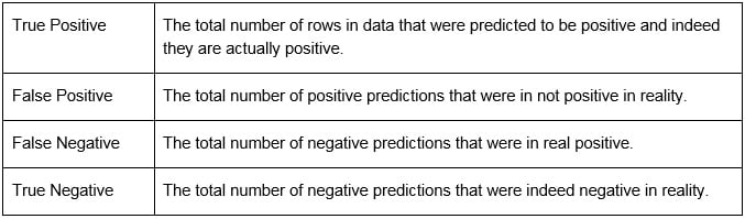
  Let's consider a classification problem that has an output value of either positive or negative. The confusion matrix provides four types of statistics in the form of a matrix for this classification problem.

Figure 1.2: Statistics in a classification problem

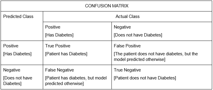
Let's take an example of patients diagnosed with diabetes. Here, the model has been trained to predict whether a patient has diabetes or not. The actual class means the actual lab result for the person. The predicted class is the predicted result from the trained model.

Figure 1.3: A confusion matrix of diabetes data

• Precision

  Precision = True positives/(True positives + False positives)

• Recall

  Recall = True positives/(True positives + False negatives)

• Mean squared error

  The difference between the original value and the predicted value is known as error. The average of the absolute square of the errors is known as the mean squared error.

• Mean absolute error

  The difference between the original value and the predicted value is known as error. The average of the errors is known as the mean absolute error.

• RMSE

  Root Mean Squared Error (RMSE) is the square root of the mean squared difference between the model predictions and the actual output values.

• ROC curve

  The Receiver Operating Characteristic (ROC) curve is a visual measure of performance for a classification problem. The curve plots true positive rate to the false positive rate.

• R-squared

  This measures the amount of variation in the output variable, which can be explained by the input variables. The greater the value, the more is the variation of output variable by the input variable.

• Adjusted R-squared

  This is used for multiple variable regression problems. It is similar to R-squared, but if the input variable added does does not improve the model's predictions, then the value of adjusted R-squared decreases.

Deployment Process

This is also the prediction phase. This is the stage where the model with optimal performance is chosen for deployment. This model will then be used on real data. The performance of the model has to be monitored and the model has to be retrained at regular intervals if required so that the prediction can be made with better accuracy for the future data.

Process Flow for Making Predictions

Imagine that you have to create a machine learning model to predict the value/price of the house by training a machine learning model. The process to do this is as follows:

1. Raw data: The input data should contain information about the house, such as its location, size, amenities, number of bedrooms, number of bathrooms, proximity to a train station, and proximity to a bus stop.
2. Data pre-processing: During the pre-processing step, we perform cleaning of the raw data; for example, handling missing values, removing outliers, and scaling the data. We then select the features from the raw data that are relevant for our house price prediction, such as location, proximity to a bus stop, and size. We would also create new features such as the amenity index, which is a weighted average of all the amenities like nearest supermarket, nearest train station, and nearest food court. This could be a value ranging from 0-1. We can also have a condition score, a combination of various factors to signify the move-in condition of the unit. Based on the physical appearance of the house, a subjective score can be given of between 0-1 for factors such as cleanliness, paint on walls, renovations done, and repairs to be done.
3. Data splitting: The data will be split into 80% for training and 20% for testing purposes.
4. Training: We can select any regression model, such as support vector regression, linear regression, and gradient boosted and implement them using R.
5. Evaluation: The models will be evaluated based on metrics such as, mean absolute error (MAE), and RMSE.
6. Deployment: The models will be compared with each other using the evaluation metrics. When the values are acceptable to us and the values do not overfit, we would proceed to deploy the model into production. This would require us to develop software to create a workflow for training, retraining, refreshing the models after retraining, and prediction on new data.

The process is now clear. Let's move on to R programming.