-
Book Overview & Buying
-
Table Of Contents

Practical Machine Learning with R
By :
Practical Machine Learning with R
By:
Overview of this book
With huge amounts of data being generated every moment, businesses need applications that apply complex mathematical calculations to data repeatedly and at speed. With machine learning techniques and R, you can easily develop these kinds of applications in an efficient way.
Practical Machine Learning with R begins by helping you grasp the basics of machine learning methods, while also highlighting how and why they work. You will understand how to get these algorithms to work in practice, rather than focusing on mathematical derivations. As you progress from one chapter to another, you will gain hands-on experience of building a machine learning solution in R. Next, using R packages such as rpart, random forest, and multiple imputation by chained equations (MICE), you will learn to implement algorithms including neural net classifier, decision trees, and linear and non-linear regression. As you progress through the book, you’ll delve into various machine learning techniques for both supervised and unsupervised learning approaches. In addition to this, you’ll gain insights into partitioning the datasets and mechanisms to evaluate the results from each model and be able to compare them.
By the end of this book, you will have gained expertise in solving your business problems, starting by forming a good problem statement, selecting the most appropriate model to solve your problem, and then ensuring that you do not overtrain it.
Table of Contents (8 chapters)
About the Book

 Free Chapter
An Introduction to Machine Learning
Data Cleaning and Pre-processing
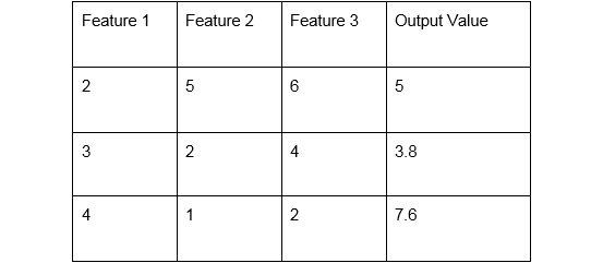
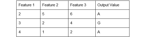
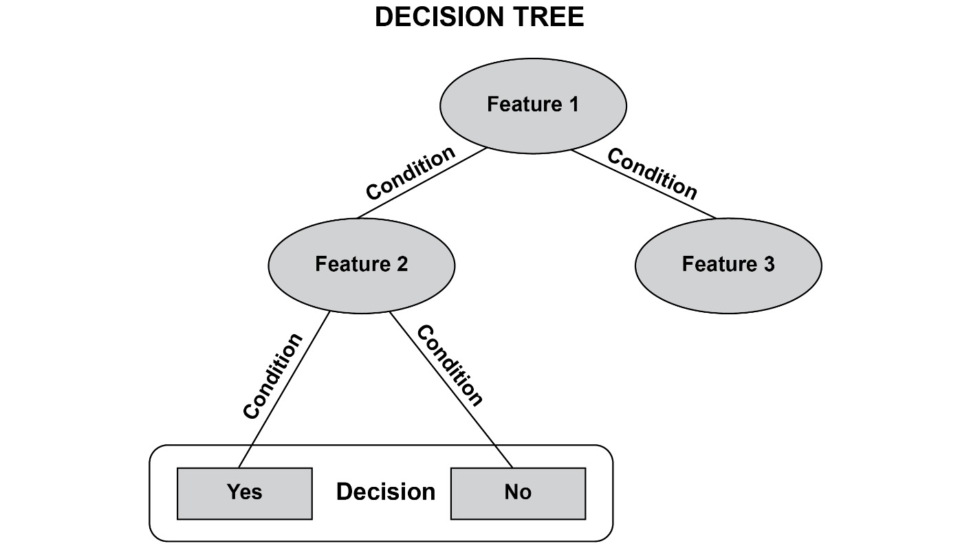
Feature Engineering
Introduction to neuralnet and Evaluation Methods
Linear and Logistic Regression Models
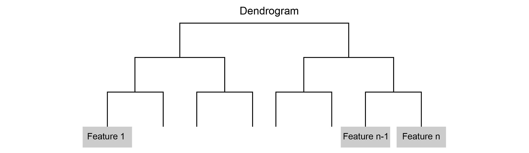
Unsupervised Learning