
Multi-layer perceptron – our first example of a network
In this chapter, we present our first example of a network with multiple dense layers. Historically, "perceptron" was the name given to a model having one single linear layer, and as a consequence, if it has multiple layers, you would call it a multi-layer perceptron (MLP). Note that the input and the output layers are visible from outside, while all the other layers in the middle are hidden – hence the name hidden layers. In this context, a single layer is simply a linear function and the MLP is therefore obtained by stacking multiple single layers one after the other:

Figure 4: An example of a multiple layer perceptron
In Figure 4 each node in the first hidden layer receives an input and "fires" (0,1) according to the values of the associated linear function. Then, the output of the first hidden layer is passed to the second layer where another linear function is applied, the results of which are passed to the final output layer consisting of one single neuron. It is interesting to note that this layered organization vaguely resembles the organization of the human vision system, as we discussed earlier.
Problems in training the perceptron and their solutions
Let's consider a single neuron; what are the best choices for the weight w and the bias b? Ideally, we would like to provide a set of training examples and let the computer adjust the weight and the bias in such a way that the errors produced in the output are minimized.
In order to make this a bit more concrete, let's suppose that we have a set of images of cats and another separate set of images not containing cats. Suppose that each neuron receives input from the value of a single pixel in the images. While the computer processes those images, we would like our neuron to adjust its weights and its bias so that we have fewer and fewer images wrongly recognized.
This approach seems very intuitive, but it requires a small change in the weights (or the bias) to cause only a small change in the outputs. Think about it: if we have a big output jump, we cannot learn progressively. After all, kids learn little by little. Unfortunately, the perceptron does not show this "little-by-little" behavior. A perceptron is either a 0 or 1, and that's a big jump that will not help in learning (see Figure 5):

Figure 5: Example of perceptron - either a 0 or 1
We need something different; something smoother. We need a function that progressively changes from 0 to 1 with no discontinuity. Mathematically, this means that we need a continuous function that allows us to compute the derivative. You might remember that in mathematics the derivative is the amount by which a function changes at a given point. For functions with input given by real numbers, the derivative is the slope of the tangent line at a point on a graph. Later in this chapter, we will see why derivatives are important for learning, when we talk about gradient descent.
Activation function – sigmoid
The sigmoid function defined as 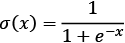 and represented in the following figure has small output changes in the range (0, 1) when the input varies in the range
  . Mathematically the function is continuous. A typical sigmoid function is represented in Figure 6:

Figure 6: A sigmoid function with output in the range (0,1)
A neuron can use the sigmoid for computing the nonlinear function 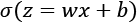 . Note that if z = wx + b is very large and positive, then
  so
so  , while if z = wx + b is very large and negative
  so
so  . In other words, a neuron with sigmoid activation has a behavior similar to the perceptron, but the changes are gradual and output values such as 0.5539 or 0.123191 are perfectly legitimate. In this sense, a sigmoid neuron can answer "maybe."
Activation function – tanh
Another useful activation function is tanh. Defined as  whose shape is shown in Figure 7, its outputs range from -1 to 1:

Figure 7: Tanh activation function
Activation function – ReLU
The sigmoid is not the only kind of smooth activation function used for neural networks. Recently, a very simple function named ReLU (REctified Linear Unit) became very popular because it helps address some optimization problems observed with sigmoids. We will discuss these problems in more detail when we talk about vanishing gradient in Chapter 9, Autoencoders. A ReLU is simply defined as f(x) = max(0, x) and the non-linear function is represented in Figure 8. As you can see, the function is zero for negative values and it grows linearly for positive values. The ReLU is also very simple to implement (generally, three instructions are enough), while the sigmoid is a few orders of magnitude more. This helped to squeeze the neural networks onto an early GPU:

Figure 8: A ReLU function
Two additional activation functions – ELU and LeakyReLU
Sigmoid and ReLU are not the only activation functions used for learning.
ELU is defined as 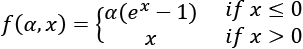 for
for  and its plot is represented in Figure 9:

Figure 9: An ELU function
LeakyReLU is defined as 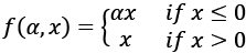 for
for  and its plot is represented in Figure 10:

Figure 10: A LeakyReLU function
Both the functions allow small updates if x is negative, which might be useful in certain conditions.
Activation functions
Sigmoid, Tanh, ELU, LeakyReLU, and ReLU are generally called activation functions in neural network jargon. In the gradient descent section, we will see that those gradual changes typical of sigmoid and ReLU functions are the basic building blocks to develop a learning algorithm that adapts little by little by progressively reducing the mistakes made by our nets. An example of using the activation function  with (x1, x2,..., xm) input vector, (w1, w2,..., wm) weight vector, b bias, and
  summation is given in Figure 11. Note that TensorFlow 2.0 supports many activation functions, a full list of which is available online:

Figure 11: An example of an activation function applied after a linear function
In short – what are neural networks after all?
In one sentence, machine learning models are a way to compute a function that maps some inputs to their corresponding outputs. The function is nothing more than a number of addition and multiplication operations. However, when combined with a non-linear activation and stacked in multiple layers, these functions can learn almost anything [8]. You also need a meaningful metric capturing what you want to optimize (this being the so-called loss function that we will cover later in the book), enough data to learn from, and sufficient computational power.
Now, it might be beneficial to stop one moment and ask ourselves what "learning" really is? Well, we can say for our purposes that learning is essentially a process aimed at generalizing established observations [9] in order to predict future results. So, in short, this is exactly the goal we want to achieve with neural networks.