
A real example – recognizing handwritten digits
In this section we will build a network that can recognize handwritten numbers. In order to achieve this goal, we'll use MNIST (http://yann.lecun.com/exdb/mnist/), a database of handwritten digits made up of a training set of 60,000 examples, and a test set of 10,000 examples. The training examples are annotated by humans with the correct answer. For instance, if the handwritten digit is the number "3", then 3 is simply the label associated with that example.
In machine learning, when a dataset with correct answers is available, we say that we can perform a form of supervised learning. In this case we can use training examples to improve our net. Testing examples also have the correct answer associated to each digit. In this case, however, the idea is to pretend that the label is unknown, let the network do the prediction, and then later on reconsider the label to evaluate how well our neural network has learned to recognize digits. Unsurprisingly, testing examples are just used to test the performance of our net.
Each MNIST image is in grayscale and consists of 28*28 pixels. A subset of these images of numbers is shown in Figure 12:

Figure 12: A collection of MNIST images
One-hot encoding (OHE)
We are going to use OHE as a simple tool to encode information used inside neural networks. In many applications it is convenient to transform categorical (non-numerical) features into numerical variables. For instance, the categorical feature "digit" with value d in [0 – 9] can be encoded into a binary vector with 10 positions, which always has 0 value except the d - th position where a 1 is present.
For example, the digit 3 can be encoded as [0, 0, 0, 1, 0, 0, 0, 0, 0, 0]. This type of representation is called One-hot encoding, or sometimes simply one-hot, and is very common in data mining when the learning algorithm is specialized in dealing with numerical functions.
Defining a simple neural network in TensorFlow 2.0
In this section, we use TensorFlow 2.0 to define a network that recognizes MNIST handwritten digits. We start with a very simple neural network and then progressively improve it.
Following Keras style, TensorFlow 2.0 provides suitable libraries (https://www.tensorflow.org/api_docs/python/tf/keras/datasets) for loading the dataset and splits it into training sets, X_train, used for fine-tuning our net, and test sets, X_test, used for assessing the performance. Data is converted into float32 to use 32-bit precision when training a neural network and normalized to the range [0,1]. In addition, we load the true labels into Y_train and Y_test respectively, and perform a one-hot encoding on them. Let's see the code.
For now, do not focus too much on understanding why certain parameters have specific assigned values, as these choices will be discussed throughout the rest of the book. Intuitively, EPOCH defines how long the training should last, BATCH_SIZE is the number of samples you feed in to your network at a time, and VALIDATION is the amount of data reserved for checking or proving the validity of the training process. The reason why we picked EPOCHS = 200, BATCH_SIZE = 128, VALIDATION_SPLIT=0.2, and N_HIDDEN = 128 will be clearer later in this chapter when we will explore different values and discuss hyperparameter optimization. Let's look at our first code fragment of a neural network in TensorFlow. Reading is intuitive but you will find a detailed explanation in the following pages:
import tensorflow as tf
import numpy as np
from tensorflow import keras
# Network and training parameters.
EPOCHS = 200
BATCH_SIZE = 128
VERBOSE = 1
NB_CLASSES = 10   # number of outputs = number of digits
N_HIDDEN = 128
VALIDATION_SPLIT = 0.2 # how much TRAIN is reserved for VALIDATION
# Loading MNIST dataset.
# verify
# You can verify that the split between train and test is 60,000, and 10,000 respectively.
# Labels have one-hot representation.is automatically applied
mnist = keras.datasets.mnist
(X_train, Y_train), (X_test, Y_test) = mnist.load_data()
# X_train is 60000 rows of 28x28 values; we  --> reshape it to
# 60000 x 784.
RESHAPED = 784
#
X_train = X_train.reshape(60000, RESHAPED)
X_test = X_test.reshape(10000, RESHAPED)
X_train = X_train.astype('float32')
X_test = X_test.astype('float32')
# Normalize inputs to be within in [0, 1].
X_train /= 255
X_test /= 255
print(X_train.shape[0], 'train samples')
print(X_test.shape[0], 'test samples')
# One-hot representation of the labels.
Y_train = tf.keras.utils.to_categorical(Y_train, NB_CLASSES)
Y_test = tf.keras.utils.to_categorical(Y_test, NB_CLASSES)
You can see from the above code that the input layer has a neuron associated to each pixel in the image for a total of 28*28=784 neurons, one for each pixel in the MNIST images.
Typically, the values associated with each pixel are normalized in the range [0,1] (which means that the intensity of each pixel is divided by 255, the maximum intensity value). The output can be one of ten classes, with one class for each digit.
The final layer is a single neuron with activation function "softmax", which is a generalization of the sigmoid function. As discussed earlier, a sigmoid function output is in the range (0, 1) when the input varies in the range  . Similarly, a softmax "squashes" a K-dimensional vector of arbitrary real values into a K-dimensional vector of real values in the range (0, 1), so that they all add up to 1. In our case, it aggregates 10 answers provided by the previous layer with 10 neurons. What we have just described is implemented with the following code:
# Build the model.
model = tf.keras.models.Sequential()
model.add(keras.layers.Dense(NB_CLASSES,
   input_shape=(RESHAPED,),
   name='dense_layer',
   activation='softmax'))
Once we define the model, we have to compile it so that it can be executed by TensorFlow 2.0. There are a few choices to be made during compilation. Firstly, we need to select an optimizer, which is the specific algorithm used to update weights while we train our model. Second, we need to select an objective function, which is used by the optimizer to navigate the space of weights (frequently, objective functions are called either loss functions or cost functions and the process of optimization is defined as a process of loss minimization). Third, we need to evaluate the trained model.
A complete list of optimizers can be found at https://www.tensorflow.org/api_docs/python/tf/keras/optimizers.
Some common choices for objective functions are:
MSE, which defines the mean squared error between the predictions and the true values. Mathematically, if d is a vector of predictions and y is the vector of n observed values, then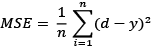 . Note that this objective function is the average of all the mistakes made in each prediction. If a prediction is far off from the true value, then this distance is made more evident by the squaring operation. In addition, the square can add up the error regardless of whether a given value is positive or negative.
binary_crossentropy, which defines the binary logarithmic loss. Suppose that our model predicts p while the target is c, then the binary cross-entropy is defined as . Note that this objective function is suitable for binary label prediction.
categorical_crossentropy, which defines the multiclass logarithmic loss. Categorical cross-entropy compares the distribution of the predictions with the true distribution, with the probability of the true class set to 1 and 0 for the other classes. If the true class is c and the prediction is y, then the categorical cross-entropy is defined as:
One way to think about multi-class logarithm loss is to consider the true class represented as a one-hot encoded vector, and the closer the model's outputs are to that vector, the lower the loss. Note that this objective function is suitable for multi-class label predictions. It is also the default choice in association with softmax activation.
A complete list of loss functions can be found at https://www.tensorflow.org/api_docs/python/tf/keras/losses.
Some common choices for metrics are:
Accuracy, which defines the proportion of correct predictions with respect to the targetsPrecision, which defines how many selected items are relevant for a multi-label classificationRecall, which defines how many selected items are relevant for a multi-label classification
A complete list of metrics can be found at https://www.tensorflow.org/api_docs/python/tf/keras/metrics.
Metrics are similar to objective functions, with the only difference that they are not used for training a model, but only for evaluating the model. However, it is important to understand the difference between metrics and objective functions. As discussed, the loss function is used to optimize your network. This is the function minimized by the selected optimizer. Instead, a metric is used to judge the performance of your network. This is only for you to run an evaluation on and it should be separated from the optimization process. On some occasions, it would be ideal to directly optimize for a specific metric. However, some metrics are not differentiable with respect to their inputs, which precludes them from being used directly.
When compiling a model in TensorFlow 2.0, it is possible to select the optimizer, the loss function, and the metric used together with a given model:
# Compiling the model.
model.compile(optimizer='SGD',
              loss='categorical_crossentropy',
              metrics=['accuracy'])
Stochastic Gradient Descent (SGD) (see Chapter 15, The Math Behind Deep Learning) is a particular kind of optimization algorithm used to reduce the mistakes made by neural networks after each training epoch. We will review SGD and other optimization algorithms in the next chapters. Once the model is compiled, it can then be trained with the fit() method, which specifies a few parameters:
epochsis the number of times the model is exposed to the training set. At each iteration the optimizer tries to adjust the weights so that the objective function is minimized.batch_sizeis the number of training instances observed before the optimizer performs a weight update; there are usually many batches per epoch.
Training a model in TensorFlow 2.0 is very simple:
# Training the model.
model.fit(X_train, Y_train,
               batch_size=BATCH_SIZE, epochs=EPOCHS,
               verbose=VERBOSE, validation_split=VALIDATION_SPLIT)
Note that we've reserved part of the training set for validation. The key idea is that we reserve a part of the training data for measuring the performance on the validation while training. This is a good practice to follow for any machine learning task, and one that we will adopt in all of our examples. Please note that we will return to validation later in this chapter when we talk about overfitting.
Once the model is trained, we can evaluate it on the test set that contains new examples never seen by the model during the training phase.
Note that, of course, the training set and the test set are rigorously separated. There is no point evaluating a model on an example that was already used for training. In TensorFlow 2.0 we can use the method evaluate(X_test, Y_test) to compute the test_loss and the test_acc:
#evaluate the model
test_loss, test_acc = model.evaluate(X_test, Y_test)
print('Test accuracy:', test_acc)
So, congratulations! You have just defined your first neural network in TensorFlow 2.0. A few lines of code and your computer should be able to recognize handwritten numbers. Let's run the code and see what the performance is.
Running a simple TensorFlow 2.0 net and establishing a baseline
So let's see what happens when we run the code:

Figure 13: Code ran from our test neural network
First, the net architecture is dumped and we can see the different types of layers used, their output shape, how many parameters (that is, how many weights) they need to optimize, and how they are connected. Then, the network is trained on 48,000 samples, and 12,000 are reserved for validation. Once the neural model is built, it is then tested on 10,000 samples. For now, we won't go into the internals of how the training happens, but we can see that the program runs for 200 iterations and each time accuracy improves. When the training ends, we test our model on the test set and we achieve about 89.96% accuracy on training, 90.70% on validation, and 90.71% on test:

Figure 14: Results from testing model, accuracies displayed
This means that nearly 1 in 10 images are incorrectly classified. We can certainly do better than that.
Improving the simple net in TensorFlow 2.0 with hidden layers
Okay, we have a baseline of accuracy of 89.96% on training, 90.70% on validation, and 90.71% on test. It is a good starting point, but we can improve it. Let's see how.
An initial improvement is to add additional layers to our network because these additional neurons might intuitively help it to learn more complex patterns in the training data. In other words, additional layers add more parameters, potentially allowing a model to memorize more complex patterns. So, after the input layer, we have a first dense layer with N_HIDDEN neurons and an activation function "ReLU." This additional layer is considered hidden because it is not directly connected either with the input or with the output. After the first hidden layer, we have a second hidden layer again with N_HIDDEN neurons followed by an output layer with 10 neurons, each one of which will fire when the relative digit is recognized. The following code defines this new network:
import tensorflow as tf
from tensorflow import keras
# Network and training.
EPOCHS = 50
BATCH_SIZE = 128
VERBOSE = 1
NB_CLASSES = 10   # number of outputs = number of digits
N_HIDDEN = 128
VALIDATION_SPLIT = 0.2 # how much TRAIN is reserved for VALIDATION
# Loading MNIST dataset.
# Labels have one-hot representation.
mnist = keras.datasets.mnist
(X_train, Y_train), (X_test, Y_test) = mnist.load_data()
# X_train is 60000 rows of 28x28 values; we reshape it to 60000 x 784.
RESHAPED = 784
#
X_train = X_train.reshape(60000, RESHAPED)
X_test = X_test.reshape(10000, RESHAPED)
X_train = X_train.astype('float32')
X_test = X_test.astype('float32')
# Normalize inputs to be within in [0, 1].
X_train, X_test = X_train / 255.0, X_test / 255.0
print(X_train.shape[0], 'train samples')
print(X_test.shape[0], 'test samples')
# Labels have one-hot representation.
Y_train = tf.keras.utils.to_categorical(Y_train, NB_CLASSES)
Y_test = tf.keras.utils.to_categorical(Y_test, NB_CLASSES)
# Build the model.
model = tf.keras.models.Sequential()
model.add(keras.layers.Dense(N_HIDDEN,
          input_shape=(RESHAPED,),
          name='dense_layer', activation='relu'))
model.add(keras.layers.Dense(N_HIDDEN,
          name='dense_layer_2', activation='relu'))
model.add(keras.layers.Dense(NB_CLASSES,
          name='dense_layer_3', activation='softmax'))
# Summary of the model.
model.summary()
# Compiling the model.
model.compile(optimizer='SGD',
              loss='categorical_crossentropy',
              metrics=['accuracy'])
# Training the model.
model.fit(X_train, Y_train,
          batch_size=BATCH_SIZE, epochs=EPOCHS,
          verbose=VERBOSE, validation_split=VALIDATION_SPLIT)
# Evaluating the model.
test_loss, test_acc = model.evaluate(X_test, Y_test)
print('Test accuracy:', test_acc)
Note that to_categorical(Y_train, NB_CLASSES) converts the array Y_train into a matrix with as many columns as there are classes. The number of rows stays the same. So, for instance if we have:
> labels
array([0, 2, 1, 2, 0])
then:
to_categorical(labels)
array([[ 1.,  0.,  0.],
       [ 0.,  0.,  1.],
       [ 0.,  1.,  0.],
       [ 0.,  0.,  1.],
       [ 1.,  0.,  0.]], dtype=float32)
Let's run the code and see what results we get with this multi-layer network:

Figure 15: Running the code for a multi-layer network
The previous screenshot shows the initial steps of the run while the following screenshot shows the conclusion. Not bad. As seen in the following screenshot, by adding two hidden layers we reached 90.81% on the training set, 91.40% on validation, and 91.18% on test. This means that we have increased accuracy on testing with respect to the previous network, and we have reduced the number of iterations from 200 to 50. That's good, but we want more.
If you want, you can play by yourself and see what happens if you add only one hidden layer instead of two or if you add more than two layers. I leave this experiment as an exercise:

Figure 16: Results after adding two hidden layers, with accuracies shown
Note that improvement stops (or they become almost imperceptible) after a certain number of epochs. In machine learning, this is a phenomenon called convergence.
Further improving the simple net in TensorFlow with Dropout
Now our baseline is 90.81% on the training set, 91.40% on validation, and 91.18% on test. A second improvement is very simple. We decide to randomly drop – with the DROPOUT probability – some of the values propagated inside our internal dense network of hidden layers during training. In machine learning this is a well-known form of regularization. Surprisingly enough, this idea of randomly dropping a few values can improve our performance. The idea behind this improvement is that random dropout forces the network to learn redundant patterns that are useful for better generalization:
import tensorflow as tf
import numpy as np
from tensorflow import keras
# Network and training.
EPOCHS = 200
BATCH_SIZE = 128
VERBOSE = 1
NB_CLASSES = 10   # number of outputs = number of digits
N_HIDDEN = 128
VALIDATION_SPLIT = 0.2 # how much TRAIN is reserved for VALIDATION
DROPOUT = 0.3
# Loading MNIST dataset.
# Labels have one-hot representation.
mnist = keras.datasets.mnist
(X_train, Y_train), (X_test, Y_test) = mnist.load_data()
# X_train is 60000 rows of 28x28 values; we reshape it to 60000 x 784.
RESHAPED = 784
#
X_train = X_train.reshape(60000, RESHAPED)
X_test = X_test.reshape(10000, RESHAPED)
X_train = X_train.astype('float32')
X_test = X_test.astype('float32')
# Normalize inputs within [0, 1].
X_train, X_test = X_train / 255.0, X_test / 255.0
print(X_train.shape[0], 'train samples')
print(X_test.shape[0], 'test samples')
# One-hot representations for labels.
Y_train = tf.keras.utils.to_categorical(Y_train, NB_CLASSES)
Y_test = tf.keras.utils.to_categorical(Y_test, NB_CLASSES)
# Building the model.
model = tf.keras.models.Sequential()
model.add(keras.layers.Dense(N_HIDDEN,
          input_shape=(RESHAPED,),
          name='dense_layer', activation='relu'))
model.add(keras.layers.Dropout(DROPOUT))
model.add(keras.layers.Dense(N_HIDDEN,
          name='dense_layer_2', activation='relu'))
model.add(keras.layers.Dropout(DROPOUT))
model.add(keras.layers.Dense(NB_CLASSES,
          name='dense_layer_3', activation='softmax'))
# Summary of the model.
model.summary()
# Compiling the model.
model.compile(optimizer='SGD',
              loss='categorical_crossentropy',
              metrics=['accuracy'])
# Training the model.
model.fit(X_train, Y_train,
          batch_size=BATCH_SIZE, epochs=EPOCHS,
          verbose=VERBOSE, validation_split=VALIDATION_SPLIT)
# Evaluating the model.
test_loss, test_acc = model.evaluate(X_test, Y_test)
print('Test accuracy:', test_acc)
Let's run the code for 200 iterations as before, and we'll see that this net achieves an accuracy of 91.70% on training, 94.42% on validation, and 94.15% on testing:

Figure 17: Further testing of the neutal network, with accuracies shown
Note that it has been frequently observed that networks with random dropout in internal hidden layers can "generalize" better on unseen examples contained in test sets. Intuitively, we can consider this phenomenon as each neuron becoming more capable because it knows it cannot depend on its neighbors. Also, because it forces information to be stored in a redundant way. During testing there is no dropout, so we are now using all our highly tuned neurons. In short, it is generally a good approach to test how a net performs when a dropout function is adopted.
Besides that, note that training accuracy should still be above test accuracy, otherwise, we might be not training for long enough. This is the case in our example and therefore we should increase the number of epochs. However, before performing this attempt we need to introduce a few other concepts that allow the training to converge faster. Let's talk about optimizers.
Testing different optimizers in TensorFlow 2.0
Now that we have defined and used a network, it is useful to start developing some intuition about how networks are trained, using an analogy. Let us focus on one popular training technique known as Gradient Descent (GD). Imagine a generic cost function C(w) in one single variable w as shown in Figure 18:

Figure 18: An example of gradient descent optimization
The gradient descent can be seen as a hiker who needs to navigate down a steep slope and aims to enter a ditch. The slope represents the function C while the ditch represents the minimum Cmin. The hiker has a starting point w0. The hiker moves little by little; imagine that there is almost zero visibility, so the hiker cannot see where to go automatically, and they proceed in a zigzag. At each step r, the gradient is the direction of maximum increase.
Mathematically this direction is the value of the partial derivative  evaluated at point wr, reached at step r. Therefore, by taking the opposite direction
  the hiker can move towards the ditch.
At each step, the hiker can decide how big a stride to take before the next stop. This is the so-called "learning rate"  in gradient descent jargon. Note that if
  is too small, then the hiker will move slowly. However, if is too high, then the hiker will possibly miss the ditch by stepping over it.
Now you should remember that a sigmoid is a continuous function and it is possible to compute the derivative. It can be proven that the sigmoid 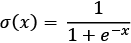 has the derivative
  .
.
ReLU is not differentiable at 0. We can however extend the first derivative at 0 to a function over the whole domain by defining it to be either a 0 or 1.
The piecewise derivative of ReLU y = max(0, x) is  . Once we have the derivative, it is possible to optimize the nets with a gradient descent technique. TensorFlow computes the derivative on our behalf so we don't need to worry about implementing or computing it.
A neural network is essentially a composition of multiple derivable functions with thousands and sometimes millions of parameters. Each network layer computes a function, the error of which should be minimized in order to improve the accuracy observed during the learning phase. When we discuss backpropagation, we will discover that the minimization game is a bit more complex than our toy example. However, it is still based on the same intuition of descending a slope to reach a ditch.
TensorFlow implements a fast variant of gradient descent known as SGD and many more advanced optimization techniques such as RMSProp and Adam. RMSProp and Adam include the concept of momentum (a velocity component), in addition to the acceleration component that SGD has. This allows faster convergence at the cost of more computation. Think about a hiker who starts to move in one direction then decides to change direction but remembers previous choices. It can be proven that momentum helps accelerate SGD in the relevant direction and dampens oscillations [10].
A complete list of optimizers can be found at https://www.tensorflow.org/api_docs/python/tf/keras/optimizers.
SGD was our default choice so far. So now let's try the other two.
It is very simple; we just need to change a few lines:
# Compiling the model.
model.compile(optimizer='RMSProp',
              loss='categorical_crossentropy', metrics=['accuracy'])
That's it. Let's test it:

Figure 19: Testing RMSProp
As you can see in the preceding screenshot, RMSProp is faster than SDG since we are able to achieve in only 10 epochs an accuracy of 97.43% on training, 97.62% on validation, and 97.64% on test. That's a significant improvement on SDG. Now that we have a very fast optimizer, let us try to significantly increase the number of epochs up to 250 and we get 98.99% accuracy on training, 97.66% on validation, and 97.77% on test:

Figure 20: Increasing the number of epochs
It is useful to observe how accuracy increases on training and test sets when the number of epochs increases (see Figure 21). As you can see, these two curves touch at about 15 epochs and therefore there is no need to train further after that point (the image is generated by using TensorBoard, a standard TensorFlow tool that will be discussed in Chapter 2, TensorFlow 1.x and 2.x):

Figure 21: An example of accuracy and loss with RMSProp
Okay, let's try the other optimizer, Adam(). Pretty simple:
# Compiling the model.
model.compile(optimizer='Adam',
              loss='categorical_crossentropy',
              metrics=['accuracy'])
As we can see, Adam() is slightly better. With Adam we achieve 98.94% accuracy on training, 97.89% on validation, and 97.82% on test with 20 iterations:

Figure 22: Testing with the Adam optimizer
One more time, let's plot how accuracy increases on training and test sets when the number of epochs increases (see Figure 23). You'll notice that by choosing Adam as an optimizer, we are able to stop after just about 12 epochs or steps:

Figure 23: An example of accuracy and loss with adam
Note that this is our fifth variant and remember that our initial baseline was at 90.71% on test. So far, we've made progressive improvements. However, gains are now more and more difficult to obtain. Note that we are optimizing with a dropout of 30%. For the sake of completeness, it could be useful to report the accuracy on the test dataset for different dropout values (see Figure 24). In this example, we selected Adam() as the optimizer. Note that choice of optimizer isn't a rule of thumb and we can get different performance depending on the problem-optimizer combination:

Figure 24: An example of changes in accuracy for different Dropout values
Increasing the number of epochs
Let's make another attempt and increase the number of epochs used for training from 20 to 200. Unfortunately, this choice increases our computation time tenfold, yet gives us no gain. The experiment is unsuccessful, but we have learned that if we spend more time learning, we will not necessarily improve the result. Learning is more about adopting smart techniques and not necessarily about the time spent in computations. Let's keep track of our five variants in the following graph (see Figure 25):

Figure 25: Accuracy for different models and optimizers
Controlling the optimizer learning rate
There is another approach we can take that involves changing the learning parameter for our optimizer. As you can see in Figure 26, the best value reached by our three experiments [lr=0.1, lr=0.01, lr=0.001] is 0.1, which is the default learning rate for the optimizer. Good! adam works well out of the box:

Figure 26: Accuracy for different learning rates
Increasing the number of internal hidden neurons
Yet another approach involves changing the number of internal hidden neurons. We report the results of the experiments with an increasing number of hidden neurons. We see that by increasing the complexity of the model, the runtime increases significantly because there are more and more parameters to optimize. However, the gains that we are getting by increasing the size of the network decrease more and more as the network grows (see Figures 27, 28, and 29). Note that increasing the number of hidden neurons after a certain value can reduce the accuracy because the network might not be able to generalize well (as shown in Figure 29):

Figure 27: Number of parameters for increasing values of internal hidden neurons

Figure 28: Seconds of computation time for increasing values of internal hidden neurons

Figure 29: Test accuracy for increasing the values of internal hidden neurons
Increasing the size of batch computation
Gradient descent tries to minimize the cost function on all the examples provided in the training sets and, at the same time, for all the features provided in input. SGD is a much less expensive variant that considers only BATCH_SIZE examples. So, let us see how it behaves when we change this parameter. As you can see, the best accuracy value is reached for a BATCH_SIZE=64 in our four experiments (see Figure 30):

Figure 30: Test accuracy for different batch values
Summarizing experiments run for recognizing handwritten charts
So, let's summarize: with five different variants, we were able to improve our performance from 90.71% to 97.82%. First, we defined a simple layer network in TensorFlow 2.0. Then, we improved the performance by adding some hidden layers. After that, we improved the performance on the test set by adding a few random dropouts in our network, and then by experimenting with different types of optimizers:
|
model/accuracy |
training | validation | test |
| simple |
89.96% |
90.70% |
90.71% |
| 2 hidden(128) |
90.81% |
91.40% |
91.18% |
| dropout(30%) |
91.70% |
94.42% |
94.15% (200 epochs) |
| RMSProp |
97.43% |
97.62% |
97.64% (10 epochs) |
| Adam |
98.94% |
97.89% |
97.82% (10 epochs) |
However, the next two experiments (not shown in the preceding table) were not providing significant improvements. Increasing the number of internal neurons creates more complex models and requires more expensive computations, but it provides only marginal gains. We have the same experience if we increase the number of training epochs. A final experiment consisted of changing the BATCH_SIZE for our optimizer. This also provided marginal results.