Machine learning is important for computer science because it allows complex functions to be modeled without them being explicitly written. Those models are automatically learned from examples, instead of being manually defined. This has a huge implication for arts in general since explicitly writing the rules of a painting or a musical score is inherently difficult.

In recent years, the advent of deep learning has propelled machine learning to new heights in terms of efficiency. Deep learning is especially important for our use case of music generation since using deep learning techniques doesn't require a preprocessing step of feature extraction, which is necessary for classical machine learning and hard to do on raw data such as image, text, and – you guessed it – audio. In other words, traditional machine learning algorithms do not work well for music generation. Therefore, all the networks in this book will be deep neural networks.

In this section, we'll learn what advances in deep learning allow for music generation and introduce the concepts we'll be using throughout this book. We'll also look at the different types of musical representations for those algorithms, which is important as it will serve as the groundwork for this book for data in general.

We all know that deep learning has recently become a fast-growing domain in computer science. Not so long ago, no deep learning algorithms could outperform standard techniques. That was before 2012 when, for the first time, a deep learning algorithm, AlexNet, did better in an image classification competition by using a deep neural network trained on GPUs (see the Further reading section for the AlexNet paper, one of the most influential papers that was published in computer vision). Neural network techniques are more than 30 years old, but the recent reemergence can be explained by the availability of massive data, efficient computing power, and technical advances.

Most importantly, a deep learning technique is general, in the sense that, as opposed to the music generation techniques we've specified previously, a machine learning system is agnostic and can learn from an arbitrary corpus of music. The same system can be used in multiple musical genres, as we'll see during this book when we train an existing model on jazz music in Chapter 6, Data Preparation for Training.

Many techniques in deep learning were discovered a long time ago but only find meaningful usage today. Of the technical advances in the field that concern music generation, those are present in Magenta and will be explained later in this book:

• Recurrent Neural Networks (RNNs) are interesting for music generation because they allow us to operate over sequences of vectors for the input and output. When using classic neural networks or convolutional networks (which are used in image classification), you are limited to a fixed size input vector to produce a fixed size output vector, which would be very limiting for music processing, but works well for certain types of image processing. The other advantage of RNN is the possibility of producing a new state vector at each pass by combining a function with the previous state vector, which a powerful mean of describing complex behavior and long-term state. We'll be talking about RNNs in Chapter 2, Generating Drum Sequences with Drums RNN.
• Long Short-Term Memory (LSTM) is an RNN with slightly different properties. It solves the problem of vanishing gradients that is present in RNNs and makes it impossible for the network to learn long-term dependencies, even if it theoretically could. The approach of using LSTM in music generation has been presented by Douglas Eck and Jurgen Schmidhuber in 2002 in a paper called Finding temporal structure in music: Blues improvisation with LSTM recurrent networks. We'll be talking about LSTM in Chapter 3, Generating Polyphonic Melodies.
• Variational autoencoders (VAEs) are analogous to classical autoencoders, in the sense that their architecture is similar, consisting of an encoder (for the input to a hidden layer), a decoder (for a hidden layer to the output), and a loss function, with the model learning to reconstruct the original input with specific constraints. The usage of VAE in generative models is recent but has shown interesting results. We'll be talking about VAE in Chapter 4, Latent Space Interpolation with Music VAE.
• Generative adversarial networks (GANs) are a class of machine learning systems where two neural networks compete with each other in a game: a generative network generates candidates while a discriminating network evaluates them. We'll be talking about GANs in Chapter 5, Audio Generation with NSynth and GANSynth.

Recent deep learning advances have profoundly changed not only music generation but also genre classification, audio transcription, note detection, composition, and more. We won't be talking about these subjects here, but they all share common ground: musical representation.

These systems can work with different representations:

• Symbolic representation, such as the MIDI (Musical Instrument Digital Interface (MIDI), describes the music using a notation containing the musical notes and timing, but not the sound or timbre of the actual sound. In general, sheet music is a good example of this. A symbolic representation of music has no sound by itself; it has to be played by instruments.
• Sub-symbolic representation, such as a raw audio waveform or a spectrogram, describes the actual sound of the music.

Different processes will require a different representation. For example, most speech recognition and synthesis models work with spectrograms, while most of the examples we will see in this book uses MIDI to generate music scores. Processes that integrate both representations are rare, but an example of this could be a score transcription that takes an audio file and translate it into MIDI or other symbolic representations.

There are other symbolic representations than MIDI, such as MusicXML and AbcNotation, but MIDI is by far the most common representation. The MIDI specification also doubles down as a protocol since it is used to carry note messages that can be used in real-time performance as well as control messages.

Let's consider some parts of a MIDI message that will be useful for this book:

• Channel [0-15]: This indicates the track that the message is sent on
• Note number [0-127]: This indicates the pitch of the note
• Velocity [0-127]: This indicates the volume of the note

To represent a musical note in MIDI, you have to send two different message types with proper timing: a Note On event, followed by a Note Off event. This implicitly defines the length of the note, which is not present in the MIDI message. This is important because MIDI was defined with live performance in mind, so using two messages – one for a keypress and another for a key release – makes sense.

From a data perspective, we'll need either need to convert MIDI notes into a format that has the note length encoded in it or keep a note on and note off approach, depending on what we're trying to do. For each model in Magenta, we'll see how the MIDI notes are encoded.

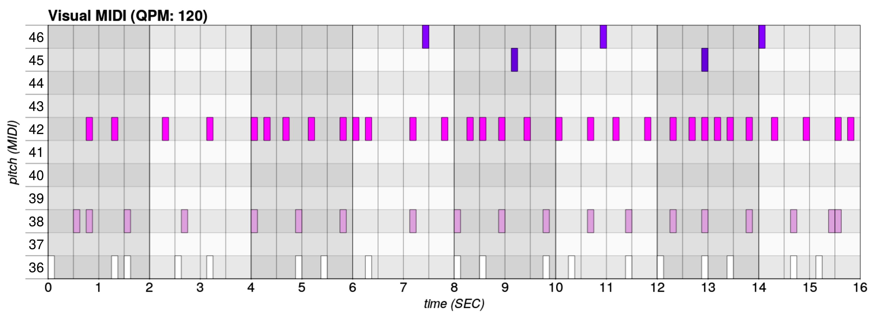
The following image shows a MIDI representation of a generated drum file, shown as a plot of time and pitch. Each MIDI note is represented by a rectangle. Because of the nature of percussion data, all the notes have the same length ("note on" followed by "note off" messages), but in general, that could vary. A drum file, by essence, is polyphonic, meaning that multiple notes can be played at the same time. We'll be talking about monophony and polyphony in the upcoming chapters.

Note that the abscissa is expressed in seconds, but it is also common to note it with bars or measures. The MIDI channel is absent from this diagram:

In the case of music generation, the majority of current deep learning systems use symbolic notation. This is also the case with Magenta. There are a couple of reasons for this:

• It is easier to represent the essence of music in terms of composition and harmony with symbolic data.
• Processing those two types of representations by using a deep learning network is similar, so choosing between both boils down to whichever is faster and more convenient. A good example of this is that the WaveNet audio generation network also has a MIDI implementation, known as the MidiNet symbolic generation network.

We'll see that the MIDI format is not directly used by Magenta, but converted into and from NoteSequence, a Protocol Buffers (Protobuf) implementation of the musical structure that is then used by TensorFlow. This is hidden from the end user since the input and output data is always MIDI. The NoteSequence implementation is useful because it implements a data format that can be used by the models for training. For example, instead of using two messages to define a note's length, a Note in a NoteSequence has a length attribute. We'll be explaining the NoteSequence implementation as we go along.

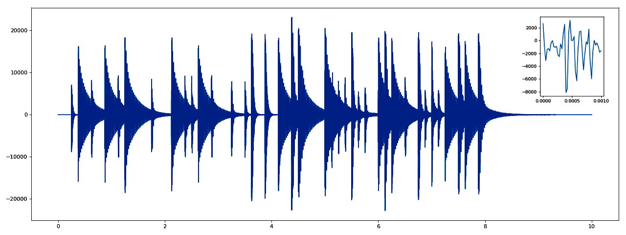
An audio waveform is a graph displaying amplitude changes over time. Zoomed out, a waveform looks rather simple and smooth, but zoomed in, we can see tiny variations – it is those variations that represent the sound.

To illustrate how a waveform works, imagine a speaker cone that's is at rest when the amplitude is at 0. If the amplitude moves to a negative value of 1, for example, then the speaker moves backward a little bit, or forward in the case of a positive value. For each amplitude variation, the speaker will move, making the air move, thus making your eardrums move.

The bigger the amplitude is in the waveform, the more the speaker cone moves in terms of distance, and the louder the sound. This is expressed in decibel (dB), a measure of sound pressure.

The faster the movement, the higher the pitch. This is expressed in hertz (Hz).

In the following image, we can see the MIDI file from the previous section played by instruments to make a WAV recording. The instrument that's being used is a 1982 Roland TR-808 drum sample pack. You can visually match some instruments, such as double the Conga Mid (MIDI note 48) at around 4.5 seconds. In the upper right corner, you can see a zoom of the waveform at 100th of a second to show the actual amplitude change:

In machine learning, using a raw audio waveform used to be uncommon as a data source since the computational load is bigger than other transformed representations, both in terms of memory and processing. But recent advances in the field, such as WaveNet models, makes it on par with other methods of representing audio, such as spectrograms, which were historically more popular for machine learning algorithms, especially for speech recognition and synthesis.

Bear in mind that training on audio is really cost-intensive because raw audio is a dense medium. Basically, a waveform is a digital recreation of a dynamic voltage over time. Simply put, a process called Pulse Code Modulation (PCM) assigns a bit value to each sample at the sampling rate you are running. The sampling rate for recording purposes is pretty standard: 44,100 Hz, which is called the Nyquist Frequency. But you don't always need a 44,100 Hz sample rate; for example, 16,000 Hz is more than enough to cover human speech frequencies. At that frequency, the first second of audio is represented by 16,000 samples.

If you want to know more about PCM, the sampling theory for audio, and the Nyquist Frequency, check out the Further reading section at the end of this chapter.

We'll look at audio representation in more detail in Chapter 5, Audio Generation with NSynth and GANSynth, since we are going to be using NSynth, a Wavenet model, to generate audio samples.

Historically, spectrograms have been a popular form of handling audio for machine learning, for two reasons – it is compact and extracting features from it is easier. To explain this, imagine the raw audio stream of the example from the previous section and cut it into chunks of 1/50th of a second (20 milliseconds) for processing. Now, you have chunks of 882 samples that are hard to represent; it is a mixed bag of amplitudes that don't really represent anything.

A spectrogram is the result of doing a Fourier transform on the audio stream. A Fourier transform will decompose a signal (a function of time) into its constituent frequencies. For an audio signal, this gives us the intensity of a frequency band, with a band being a small split of the whole spectrum, for example, 50 Hz. After applying a Fourier transform on our previous example and taking sample 1 of the 882 samples, we'll end up with the intensity for each frequency band:

• [0 Hz - 50 Hz]: a₁
• [50 Hz - 100 Hz]: a₂
• ...
• [22000 Hz - 22050 Hz:]: a_n

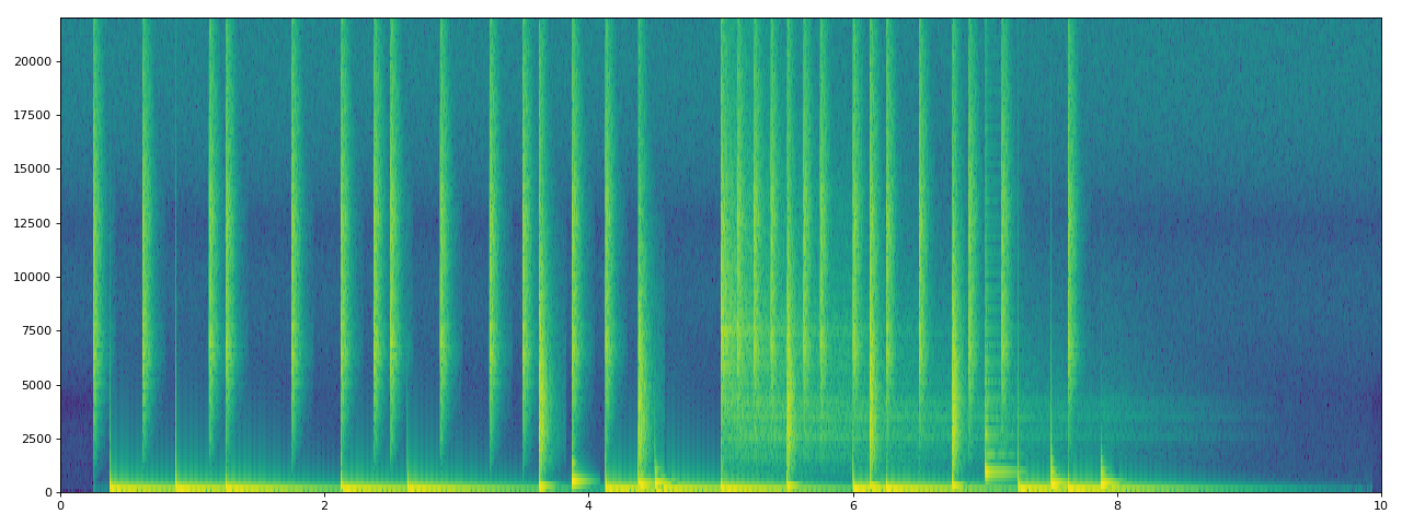
You'll end up with intensity [a₁, a₂, ..., a_n] for each band of 50 Hz up to 22,050, which is the y-axis, with an assigned color spectrum for smaller to bigger intensities. Repeating that for each 20 ms on the x-axis until the whole audio is covered gives you a spectrogram. What is interesting in a spectrogram is that you can actually see the content of the music. If a C major chord is played, you'll see C, E, and G emerge in the spectrogram at their corresponding frequency.

The following spectrogram has been generated from the waveform of the previous section. From this, you can clearly see the frequencies that are being played by the TR 808 from the given MIDI file. You should be able to visually match the waveform from the previous section with the spectrogram:

Spectrograms are mainly used in speech recognition. They are also used in speech synthesis: first, a model is trained on spectrograms aligned with text, and from there, the model will be able to produce a spectrogram that corresponds to a given text. The Griffin-Lim algorithm is used to recover an audio signal from a spectrogram.

We won't be using spectrograms in this book, but knowing how they work and what they are used for is important since they are used in many applications.

So far, we have learned which deep learning technical advances are important in music generation and learned about music representation in those algorithms. These two topics are important because we'll be looking at them throughout this book.

In the next section, we'll introduce Magenta, where you'll see much of this section's content come into play.