
Generating faces with a probabilistic model
Alright, enough mathematics. It is now time to get your hands dirty and generate your first image. In this section, we will learn how to generate images by sampling from a probabilistic model without even using a neural network.
Mean faces
We will be using the large-scale CelebFaces Attributes (CelebA) dataset created by The Chinese University of Hong Kong (http://mmlab.ie.cuhk.edu.hk/projects/CelebA.html). This can be downloaded directly with Python's tensorflow_datasets module within the ch1_generate_first_image.ipynb Jupyter notebook, as shown in the following code:
import tensorflow_datasets as tfds
import matplotlib.pyplot as plt
import numpy as np
ds_train, ds_info = tfds.load('celeb_a', split='test',
                               shuffle_files=False,
                               with_info=True)
fig = tfds.show_examples(ds_info, ds_train)
The TensorFlow dataset allows us to preview some examples of images by using the tfds.show_examples() API. The following are some samples of male and female celebrities' faces:
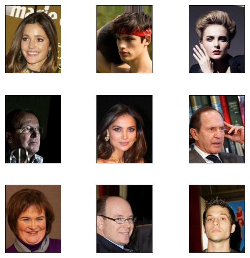
Figure 1.3 – Sample images from the CelebA dataset
As you can see in the figure, there is a celebrity face in every image. Every picture is unique, with a variety of genders, poses, expressions, and hairstyles; some wear glasses and some don't. Let's see how to exploit the probability distribution of the images to help us create a new face. We'll use one of the simplest statistical methods – the mean, which means taking an average of the pixels from the images. To be more specific, we are averaging the xi of every image to calculate the xi of a new image. To speed up the processing, we'll use only 2,000 samples from the dataset for this task, as follows:
sample_size = 2000
ds_train = ds_train.batch(sample_size)
features = next(iter(ds_train.take(1)))
sample_images = features['image']
new_image = np.mean(sample_images, axis=0)
plt.imshow(new_image.astype(np.uint8))
Ta-dah! That is your first generated image, and it looks pretty amazing! I initially thought it would look a bit like one of Picasso's paintings, but it turns out that the mean image is quite coherent:
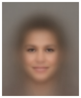
Figure 1.4 – The mean face
Conditional probability
The best thing about the CelebA dataset is that each image is labeled with facial attributes as follows:
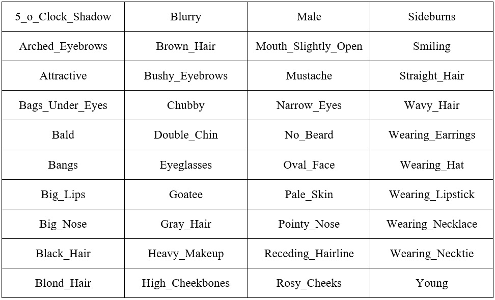
Figure 1.5 – 40 attributes in the CelebA dataset in alphabetical order
We are going to use these attributes to generate a new image. Let's say we want to generate a male image. How do we do that? Instead of calculating the probability of every image, we use only images that have the Male attribute set to true. We can put it in this way:
p(x | y)
We call this the probability of x conditioned on y, or more informally the probability of x given y. This is called conditional probability. In our example, y is the facial attributes. When we condition on the Male attribute, this variable is no longer a random probability; every sample will have the Male attribute and we can be certain that every face belongs to a man. The following figure shows new mean faces generated using other attributes as well as Male, such as Male + Eyeglasses and Male + Eyeglasses + Mustache + Smiling. Notice that as the conditions increase, the number of samples reduces and the mean image also becomes noisier:
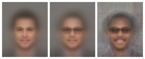
Figure 1.6 – Adding attributes from left to right. (a) Male (b) Male + Eyeglasses (c) Male + Eyeglasses + Mustache + Smiling
You could use the Jupyter notebook to generate a new face by using different attributes, but not every combination produces satisfactory results. The following are some female faces generated with different attributes. The rightmost image is an interesting one. I used attributes of Female, Smiling, Eyeglasses, and Pointy_Nose, but it turns out that people with these attributes tend to also have wavy hair, which is an attribute that was excluded in this sample. Visualization can be a useful tool to provide insights into your dataset:
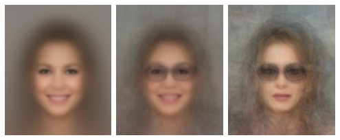
Figure 1.7 – Female faces with different attributes
Tips
Instead of using the mean when generating images, you can try to using the median as well, which may produce a sharper image. Simply replace np.mean() with np.median().
Probabilistic generative models
There are three main goals that we wish to achieve with image-generation algorithms:
- Generate images that look like ones in the given dataset.
- Generate a variety of images.
- Control the images being generated.
By simply taking the mean of the pixels in an image, we have demonstrated how to achieve goals 1 and 3. However, one limitation is that we could only generate one image per condition. That really isn't very effective for an algorithm, generating only one image from hundreds or thousands of training images.
The following chart shows the distribution of one color channel of an arbitrary pixel in the dataset. The x mark on the chart is the median value. When we use the mean or median of data, we are always sampling the same point, and therefore there is no variation in the outcome. Is there a way to generate multiple different faces? Yes, we can try to increase the generated image variation by sampling from the entire pixel distribution:
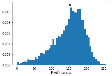
Figure 1.8 – The distribution of a pixel's color channel
A machine learning textbook will probably ask you to first create a probabilistic model, pmodel, by calculating the joint probability of every single pixel. But as the sample space is huge (remember, one RGB pixel can have 16,777,216 different values), it is computationally expensive to implement. Also, because this is a hands-on book, we will draw pixel samples directly from datasets. To create an x0 pixel in a new image, we randomly sample from an x0 pixel of all images in the dataset by running the following code:
new_image = np.zeros(sample_images.shape[1:], dtype=np.uint8)
for i in range(h):
    for j in range(w):
        rand_int = np.random.randint(0, sample_images.shape[0])
        new_image[i,j] = sample_images[rand_int,i,j]
Images were generated using random sampling. Disappointingly, although there is some variation between the images, they are not that different from each other, and one of our objectives is to be able to generate a variety of faces. Also, the images are noticeably noisier than when using the mean. The reason for this is that the pixel distribution is independent of each other.
For example, for a given pixel in the lips, we can reasonably expect the color to be pink or red, and the same goes for the adjacent pixels. Nevertheless, because we are sampling independently from images where faces appear in different locations and poses, this results in color discontinuities between pixels, ultimately giving this noisy result:
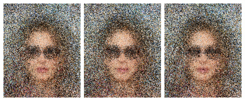
Figure 1.9 – Images generated by random sampling
Tips
You may be wondering why the mean face looks smoother than with random sampling. Firstly, it is because the distance of the mean between pixels is smaller. Imagine a random sampling scenario where one pixel sampled is close to 0 and the next one is close to 255. The mean of these pixels would likely lie somewhere in the middle, and therefore the difference between them would be smaller. On the other hand, pixels in the backgrounds of pictures tend to have a uniform distribution; for example, they could all be part of a blue sky, a white wall, green leaves, and so on. As they are distributed rather evenly across the color spectrum, the mean value is around [127, 127, 127], which happens to be gray.
Parametric modeling
What we just did was use a pixel histogram as our pmodel, but there are a few shortcomings here. Firstly, due to the large sample space, not every possible color exists in our sample distribution. As a result, the generated image will never contain any colors that are not present in the dataset. For instance, we want to be able to generate the full spectrum of skin tones rather than only one very specific shade of brown that exists in the dataset. If you did try to generate faces using conditions, you will have found that not every combination of conditions is possible. For example, for Mustache + Sideburns + Heavy_Makeup + Wavy_Hair, there simply wasn't a sample that met those conditions!
Secondly, the sample spaces increase as we increase the size of the dataset or the image resolution. This can be solved by having a parameterized model. The vertical bar chart in the following figure shows a histogram of 1,000 randomly generated numbers:
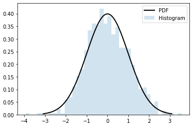
Figure 1.10 – Gaussian histogram and model
We can see that there are some bars that don't have any value. We can fit a Gaussian model on the data in which the Probability Density Function (PDF) is plotted as a black line. The PDF equation for a Gaussian distribution is as follows:
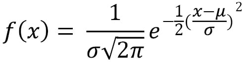
Here, µ is the mean and σ is the standard deviation.
We can see that the PDF covers the histogram gap, which means we can generate a probability for the missing numbers. This Gaussian model has only two parameters – the mean and the standard variation.
The 1,000 numbers can now be condensed to just two parameters, and we can use this model to draw as many samples as we wish; we are no longer limited to the data we fit the model with. Of course, natural images are complex and could not be described by simple models such as a Gaussian model, or in fact any mathematical models. This is where neural networks come into play. Now we will use a neural network as a parameterized image-generation model where the parameters are the network's weights and biases.