Implementing backpropagation

In feedforward propagation, we connected the input layer to the hidden layer, which then was connected to the output layer. In the first iteration, we initialized weights randomly and then calculated the loss resulting from those weight values. In backpropagation, we take the reverse approach. We start with the loss value obtained in feedforward propagation and update the weights of the network in such a way that the loss value is minimized as much as possible.

The loss value is reduced as we perform the following steps:

1. Change each weight within the neural network by a small amount – one at a time.
2. Measure the change in loss () when the weight value is changed ().
3. Update the weight by (where k is a positive value and is a hyperparameter known as the learning rate).

If the preceding steps are performed n number of times on the entire dataset (where we have done both the feedforward propagation and backpropagation), it essentially results in training for n epochs.

As a typical neural network contains thousands/millions (if not billions) of weights, changing the value of each weight, and checking whether the loss increased or decreased is not optimal. The core step in the preceding list is the measurement of "change of loss" when the weight is changed. As you might have studied in calculus, measuring this is the same as computing the gradient of loss concerning the weight. There's more on leveraging partial derivatives from calculus to calculate the gradient of the loss concerning the weight in the next section, on the chain rule for backpropagation.

In this section, we will implement gradient descent from scratch by updating one weight at a time by a small amount as detailed at the start of this section. However, before implementing backpropagation, let's understand one additional detail of neural networks: the learning rate.

Intuitively, the learning rate helps in building trust in the algorithm. For example, when deciding on the magnitude of the weight update, we would potentially not change the weight value by a big amount in one go but update it more slowly.

This results in obtaining stability in our model; we will look at how the learning rate helps with stability in the Understanding the impact of the learning rate section.

This whole process by which we update weights to reduce errors is called gradient descent.

Stochastic gradient descent is how errors are minimized in the preceding scenario. As mentioned earlier, gradient stands for the difference (which is the difference in loss values when the weight value is updated by a small amount) and descent means to reduce. Stochastic stands for the selection of random samples based on which a decision is taken.

Apart from stochastic gradient descent, many other similar optimizers help to minimize loss values; the different optimizers will be discussed in the next chapter.

In the next two sections, we will learn about coding the intuition for backpropagation from scratch in Python, and will also discuss in brief how backpropagation works using the chain rule.

Gradient descent in code

Gradient descent is implemented in Python as follows:

1. Define the feedforward network and calculate the mean squared error loss value as we did in the Feedforward propagation in code section:

from copy import deepcopy
import numpy as np
def feed_forward(inputs, outputs, weights): 
    pre_hidden = np.dot(inputs,weights[0])+ weights[1]
    hidden = 1/(1+np.exp(-pre_hidden))
    pred_out = np.dot(hidden, weights[2]) + weights[3]
    mean_squared_error = np.mean(np.square(pred_out \
                                           - outputs)) 
    return mean_squared_error

2. Increase each weight and bias value by a very small amount (0.0001) and calculate the overall squared error loss value one at a time for each of the weight and bias updates.

• In the following code, we are creating a function named update_weights, which performs the gradient descent process to update weights. The inputs to the function are the input variables to the network – inputs, expected outputs, weights (which are randomly initialized at the start of training the model), and the learning rate of the model – lr (more on the learning rate in a later section):

def update_weights(inputs, outputs, weights, lr):

• Ensure that you deepcopy the list of weights. As the weights will be manipulated in later steps, deepcopy ensures we can work with multiple copies of weights without disturbing actual weights. We will create three copies of the original set of weights that were passed as an input to the function – original_weights, temp_weights, and updated_weights:

original_weights = deepcopy(weights)
temp_weights = deepcopy(weights)
updated_weights = deepcopy(weights)           

• Calculate the loss value (original_loss) with the original set of weights by passing inputs, outputs, and original_weights through the feed_forward function:

original_loss = feed_forward(inputs, outputs, \
                                 original_weights)

• We will loop through all the layers of the network:

for i, layer in enumerate(original_weights):

• There are a total of four lists of parameters within our neural network – two lists for the weight and bias parameters that connect the input to the hidden layer and another two lists for the weight and bias parameters that connect the hidden layer to the output layer. Now, we loop through all the individual parameters and because each list has a different shape, we leverage np.ndenumerate to loop through each parameter within a given list:

for index, weight in np.ndenumerate(layer):

• Now we store the original set of weights in temp_weights. We select its index weight present in the i^th layer and increase it by a small value. Finally, we compute the new loss with the new set of weights for the neural network:

temp_weights = deepcopy(weights)
temp_weights[i][index] += 0.0001
_loss_plus = feed_forward(inputs, outputs, \
                            temp_weights)

In the first line of the preceding code, we are resetting temp_weights to the original set of weights, as in each iteration, we update a different parameter to calculate the loss when a parameter is updated by a small amount within a given epoch.

• We calculate the gradient (change in loss value) due to the weight change:

grad = (_loss_plus - original_loss)/(0.0001)

• Finally, we update the parameter present in the corresponding i^th layer and index, of updated_weights. The updated weight value will be reduced in proportion to the value of the gradient. Further, instead of completely reducing it by a value equal to the gradient value, we bring in a mechanism to build trust slowly by using the learning rate – lr (more on learning rate in the Understanding the impact of the learning rate section):

updated_weights[i][index] -= grad*lr

• Once the parameter values across all layers and indices within layers are updated, we return the updated weight values – updated_weights:

return updated_weights, original_loss

One of the other parameters in a neural network is the batch size considered in calculating the loss values.

In the preceding scenario, we considered all the data points to calculate the loss (mean squared error) value. However, in practice, when we have thousands (or in some cases, millions) of data points, the incremental contribution of a greater number of data points while calculating the loss value would follow the law of diminishing returns, and hence we would be using a batch size that is much smaller compared to the total number of data points we have. We will apply gradient descent (after feedforward propagation) using one batch at a time until we exhaust all data points within one epoch of training.

The typical batch size considered in building a model is anywhere between 32 and 1,024.

In this section, we learned about updating weight values based on the change in loss values when the weight values are changed by a small amount. In the next section, we will learn about how weights can be updated without computing gradients one gradient at a time.

Implementing backpropagation using the chain rule

So far, we have calculated gradients of loss concerning weight by updating the weight by a small amount and then calculating the difference between the feedforward loss in the original scenario (when the weight was unchanged) and the feedforward loss after updating weights. One drawback of updating weight values in this manner is that when the network is large, a large number of computations are needed to calculate loss values (and in fact, the computations are to be done twice – once where weight values are unchanged and again where weight values are updated by a small amount). This results in more computations and hence requires more resources and time. In this section, we will learn about leveraging the chain rule, which does not require us to manually compute loss values to come up with the gradient of the loss concerning the weight value.

In the first iteration (where we initialized weights randomly), the predicted value of the output is 1.235.

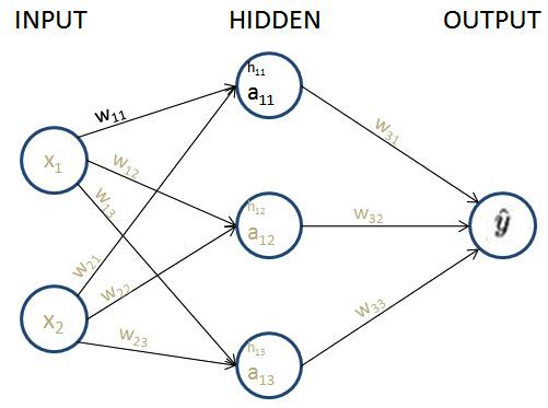
In order to get the theoretical formulation, let's denote the weights and hidden layer values and hidden layer activations as w, h, and a respectively as follows:

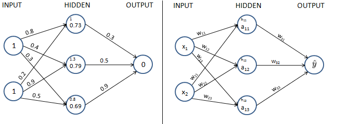
Note that, in the preceding diagrams, we have taken each component value of the left diagram and generalized it in the diagram on right.

In order to keep it easy to comprehend, in this section, we will understand how to use the chain rule to compute the gradient of loss value with respect to only w₁₁. The same learning can be extended to all the weights and biases of the neural network. We encourage you to practice and apply the chain rule calculation to the rest of the weights and bias values.

Additionally, in order to keep this simple for our learning purposes, we will be working on only one data point, where the input is {1,1} and the expected output is {0}.

Given that we are calculating the gradient of loss value with w₁₁, let's understand all the intermediate components that are to be included while calculating the gradient through the following diagram (the components that do not connect the output to w₁₁ are grayed out in the following diagram):

From the preceding diagram, we can see that w₁₁ is contributing to the loss value through the path that is highlighted, – , , and .

Next, let's formulate how , , and are obtained individually.

The loss value of the network is represented as follows:

The predicted output value is calculated as follows:

The hidden layer activation value (sigmoid activation) is calculated as follows:

The hidden layer value is calculated as follows:

Now that we have formulated all the equations, let's calculate the impact of the change in the loss value (C) with respect to the change in weight as follows:

This is called a chain rule. Essentially, we are performing a chain of differentiations to fetch the differentiation of our interest.

Note that, in the preceding equation, we have built a chain of partial differential equations in such a way that we are now able to perform partial differentiation on each of the four components individually and ultimately calculate the derivative of the loss value with respect to weight value .

The individual partial derivatives in the preceding equation are computed as follows:

• The partial derivative of the loss value with respect to the predicted output value is as follows:

• The partial derivative of the predicted output value with respect to the hidden layer activation value is as follows:

• The partial derivative of the hidden layer activation value with respect to the hidden layer value prior to activation is as follows:

Note that the preceding equation comes from the fact that the derivative of the sigmoid function is .

• The partial derivative of the hidden layer value prior to activation with respect to the weight value is as follows:

With this in place, the gradient of the loss value with respect to is calculated by replacing each of the partial differentiation terms with the corresponding value as calculated in the previous steps as follows:

From the preceding formula, we can see that we are now able to calculate the impact on the loss value of a small change in the weight value (the gradient of the loss with respect to weight) without brute-forcing our way by recomputing the feedforward propagation again.

Next, we will go ahead and update the weight value as follows:

In gradient descent, we performed the weight update process sequentially (one weight at a time). By leveraging the chain rule, we learned that there is an alternative way to calculate the impact of a change in weight by a small amount on the loss value, however, with an opportunity to perform computations in parallel.

Now that we have a solid understanding of backpropagation, both from an intuition perspective and also by leveraging the chain rule, in the next section, we will learn about how feedforward and backpropagation work together to arrive at the optimal weight values.