Solving a full MDP and, hence, the full RL problem first requires us to understand values and how we calculate the value of a state with a value function. Recall that the value function was a primary element of the RL system. Instead of using a full MDP to explain this, we instead rely on a simpler single-state problem known as the multi-armed bandit problem. This is named after the one-armed slot machines often referred to as bandits by their patrons but, in this case, the machine has multiple arms. That is, we now consider a single-state or stationary problem with multiple actions that lead to terminal states providing constant rewards. More simply, our agent is going to play a multi-arm slot machine that will give either a win or loss based on the arm pulled, with each arm always returning the same reward. An example of our agent playing this machine is shown here:

We can consider the value for a single state to be dependent on the next action, provided we also understand the reward provided by that action. Mathematically, we can define a simple value equation for learning like so:

In this equation, we have the following:

• V(a): the value for a given action
• a: action
• α: alpha or the learning rate
• r: reward

Notice the addition of a new variable called α (alpha) or the learning rate. This learning rate denotes how fast the agent needs to learn the value from pull to pull. The smaller the learning rate (0.1), the slower the agent learns. This method of action-value learning is fundamental to RL. Let's code up this simple example to solidify further in the next section.

Since this is our first example, make sure your Python environment is set to go. Again for simplicity, we prefer Anaconda. Make sure you are comfortable coding with your chosen IDE and open up the code example, Chapter_1_1.py, and follow along:

1. Let's examine the first section of the code, as shown here:

import random

reward = [1.0, 0.5, 0.2, 0.5, 0.6, 0.1, -.5]
arms = len(reward)
episodes = 100
learning_rate = .1
Value = [0.0] * arms
print(Value)

2. We first start by doing import of random. We will use random to randomly select an arm during each training episode.
3. Next, we define a list of rewards, reward. This list defines the reward for each arm (action) and hence defines the number of arms/actions on the bandit.
4. Then, we determine the number of arms using the len() function.
5. After that, we set the number of training episodes our agent will use to evaluate the value of each arm.
6. Set the learning_rate value to .1. This means the agent will learn slowly the value of each pull.
7. Next, we initialize the value for each action in a list called Value, using the following code:

Value = [0.0] * arms

8. Then, we print the Value list to the console, making sure all of the values are 0.0.

The first section of code initialized our rewards, number of arms, learning rate, and value list. Now, we need to implement the training cycle where our agent/algorithm will learn the value of each pull. Let's jump back into the code for Chapter_1_1.py and look to the next section:

1. The next section of code in the listing we want to focus on is entitled agent learns and is shown here for reference:

# agent learns
for i in range(0, episodes):
    action = random.randint(0,arms-1)
    Value[action] = Value[action] + learning_rate * (
        reward[action] - Value[action])

print(Value)

2. We start by first defining a for loop that loops through 0 to our number of episodes. For each episode, we let the agent pull an arm and use the reward from that pull to update its determination of value for that action or arm.
3. Next, we want to determine the action or arm the agent pulls randomly using the following code:

action = random.randint(0,arms-1)

4. The code just selects a random arm/action number based on the total number of arms on the bandit (minus one to allow for proper indexing).
5. This then allows us to determine the value of the pull by using the next line of code, which mirrors very well our previous value equation:

Value[action] = Value[action] + learning_rate * (       reward[action] - Value[action])

6. That line of code clearly resembles the math for our previous Value equation. Now, think about how learning_rate is getting applied during each iteration of an episode. Notice that, with a rate of .1, our agent is learning or applying 1/10^th of what reward the agent receives minus the Value function the agent previously equated. This little trick has the effect of averaging out the values across the episodes.
7. Finally, after the looping completes and all of the episodes are run, we print the updated Value function for each action.
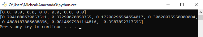
8. Run the code from the command line or your favorite Python editor. In Visual Studio, this is as simple as hitting the play button. After the code has completed running, you should see something similar to the following, but not the exact output:

Now, think back and compare those output values to the rewards set for each arm. Are they the same or different and if so, by how much? Generally, the learned values after only 100 episodes should indicate a clear value but likely not the finite value. This means the values will be smaller than the final rewards but they should still indicate a preference.

The solution we show here is an example of trial and error learning; it's that first thread we talked about back in the history of RL section. As you can see, the agent learns by randomly pulling an arm and determining the value. However, at no time does our agent learn to make better decisions based on those updated values. The agent always just pulls randomly. Our agent currently has no decision mechanism or what we call a policy in RL. We will look at how to implement a basic greedy policy in the next section.

Our current value learner is not really learning aside from finding the optimum calculated value or the reward for each action over several episodes. Since our agent is not learning, it also makes it a less efficient learner as well. After all, the agent is just randomly picking any arm each episode when it could be using its acquired knowledge, which is the Value function, to determine it's next best choice. We can code this up in a very simple policy called a greedy policy in the next exercise:

1. Open up the Chapter_1_2.py example. The code is basically the same as our last example except for the episode iteration and, in particular, the selection of action or arm. The full listing can be seen here—note the new highlighted sections:

import random

reward = [1.0, 0.5, 0.2, 0.5, 0.6, 0.1, -.5]
arms = len(reward)
learning_rate = .1
episodes = 100
Value = [0.0] * arms
print(Value)

def greedy(values):
    return values.index(max(values))

# agent learns
for i in range(0, episodes):
    action = greedy(Value)
    Value[action] = Value[action] + learning_rate * (
        reward[action] - Value[action])

print(Value)

2. Notice the inclusion of a new greedy() function. This function will always select the action with the highest value and return the corresponding index/action index. This function is essentially our agent's policy.
3. Scrolling down in the code, notice inside the training loop how we are now using the greedy() function to select our action, as shown here:

action = greedy(Value)

4. Again, run the code and look at the output. Is it what you expected? What went wrong?

Looking at your output likely shows that the agent calculated the maximum reward arm correctly, but likely didn't determine the correct values for the other arms. The reason for this is that, as soon as the agent found the most valuable arm, it kept pulling that arm. Essentially the agent finds the best path and sticks with it, which is okay in this single step or stationary environment but certainly won't work over a many step problem requiring multiple decisions. Instead, we need to balance the agents need to explore and find new paths, versus maximizing the immediate optimum reward. This problem is called the exploration versus exploitation dilemma in RL and something we will explore in the next section.

As we have seen, having our agent always make the best choice limits their ability to learn the full values of a single state never mind multiple connected states. This also severely limits an agent's ability to learn, especially in environments where multiple states converge and diverge. What we need, therefore, is a way for our agent to choose an action based on a policy that favors more equal action/value distribution. Essentially, we need a policy that allows our agent to explore as well as exploit its knowledge to maximize learning. There are multiple variations and ways of balancing the trade-off between exploration and exploitation. Much of this will depend on the particular environment as well as the specific RL implementation you are using. We would never use an absolute greedy policy but, instead, some variation of greedy or another method entirely. In our next exercise, we show how to implement an initial optimistic value method, which can be effective:

1. Open Chapter_1_3.py and look at the highlighted lines shown here:

episodes = 10000
Value = [5.0] * arms

2. First, we have increased the number of episodes to 10000. This will allow us to confirm that our new policy is converging to some appropriate solution.

3. Next, we set the initial value of the Value list to 5.0. Note that this value is well above the reward value maximum of 1.0. Using a higher value than our reward forces our agent to always explore the most valuable path, which now becomes any path it hasn't explored, hence ensuring our agent will always explore each action or arm at least once.
4. There are no more code changes and you can run the example as you normally would. The output of the example is shown here:

Your output may vary slightly but it likely will show very similar values. Notice how the calculated values are now more relative. That is, the value of 1.0 clearly indicates the best course of action, the arm with a reward of 1.0, but the other values are less indicative of the actual reward. Initial option value methods are effective but will force an agent to explore all paths, which are not so efficient in larger environments. There are of course a multitude of other methods you can use to balance exploration versus exploitation and we will cover a new method in the next section, where we introduce solving the full RL problem with Q-learning.