Sage has sophisticated plotting capabilities. By combining the power of the Python programming language with Sage's graphics functions, we can construct detailed illustrations. To demonstrate a few of Sage's advanced plotting features, we will solve a simple system of equations algebraically:

var('x')
f(x) = x^2
g(x) = x^3 - 2 * x^2 + 2

solutions=solve(f == g, x, solution_dict=True)

for s in solutions:
    show(s)

The result is as follows:

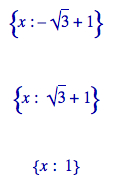
We used the keyword argument solution_dict=True to tell the solve function to return the solutions in the form of a Python list of Python dictionaries. We then used a for loop to iterate over the list and display the three solution dictionaries. We'll go into more detail about lists and dictionaries in Chapter 4. Let's illustrate our answers with a detailed plot:

p1 = plot(f, (x, -1, 3), color='blue', axes_labels=['x', 'y'])
p2 = plot(g, (x, -1, 3), color='red')

labels = []
lines = []
markers = []
for s in solutions:
    x_value = s[x].n(digits=3)
    y_value = f(x_value).n(digits=3)
    labels.append(text('y=' + str(y_value), (x_value+0.5, 
        y_value+0.5), color='black'))
    lines.append(line([(x_value, 0), (x_value, y_value)], 
        color='black', linestyle='--'))
    markers.append(point((x_value,y_value), color='black', size=30))

show(p1+p2+sum(labels) + sum(lines) + sum(markers))

The plot looks like this:

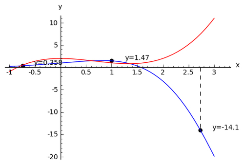
We created a plot of each function in a different colour, and labelled the axes. We then used another for loop to iterate through the list of solutions and annotate each one. Plotting will be covered in detail in Chapter 6.

Visualising a three-dimensional surface

Sage does not restrict you to making plots in two dimensions. To demonstrate the 3D capabilities of Sage, we will create a parametric plot of a mathematical surface known as the "figure 8" immersion of the Klein bottle. You will need to have Java enabled in your web browser to see the 3D plot.

var('u,v')
r = 2.0
f_x = (r + cos(u / 2) * sin(v) - sin(u / 2) 
    * sin(2 * v)) * cos(u)
f_y = (r + cos(u / 2) * sin(v) - sin(u / 2)
    * sin(2 * v)) * sin(u)
f_z = sin(u / 2) * sin(v) + cos(u / 2) * sin(2 * v)
parametric_plot3d([f_x, f_y, f_z], (u, 0, 2 * pi), 
    (v, 0, 2 * pi), color="red")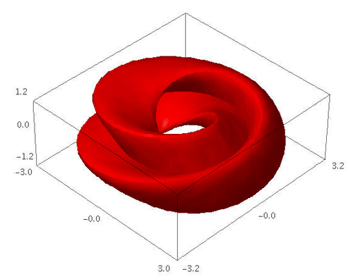

In the Sage notebook interface, the 3D plot is fully interactive. Clicking and dragging with the mouse over the image changes the viewpoint. The scroll wheel zooms in and out, and right-clicking on the image brings up a menu with further options.