

Let's plot some simple functions. Enter the following code:
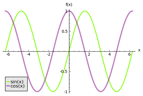
p1 = plot(sin, (-2*pi, 2*pi), thickness=2.0, rgbcolor=(0.5, 1, 0),
    legend_label='sin(x)')
p2 = plot(cos, (-2*pi, 2*pi), thickness=3.0, color='purple',
    alpha=0.5, legend_label='cos(x)')
plt = p1 + p2
plt.axes_labels(['x', 'f(x)'])

show(plt)
If you run the code from the interactive shell, the plot will open in a separate window. If you run it from the notebook interface, the plot will appear below the input cell. In either case, the result should look like this:
T
his example demonstrated the most basic type of plotting in Sage. The plot function requires the following arguments:
graphics_object = plot(callable symbolic expression, (independent_var, ind_var_min, ind_var_max))
The first argument is a callable symbolic expression, and the second argument is a tuple consisting of the independent variable, the lower limit of the domain, and the upper limit. If there...