

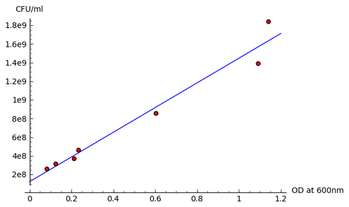
The optical density is correlated to the concentration of bacteria in the liquid. To quantify this correlation, someone has measured the optical density of a number of calibration standards of known concentration. In this example, we will fit a "standard curve" to the calibration data that we can use to determine the concentration of bacteria from optical density readings:
import numpy
var('OD, slope, intercept')
def standard_curve(OD, slope, intercept):
"""Apply a linear standard curve to optical density data"""
return OD * slope + intercept
# Enter data to define standard curve
CFU = numpy.array([2.60E+08, 3.14E+08, 3.70E+08, 4.62E+08,
8.56E+08, 1.39E+09, 1.84E+09])
optical_density = numpy.array([0.083, 0.125, 0.213, 0.234,
0.604, 1.092, 1.141])
OD_vs_CFU = zip(optical_density, CFU)
# Fit linear standard
std_params = find_fit(OD_vs_CFU, standard_curve,
parameters=[slope, intercept],
variables=[OD], initial_guess=[1e9, 3e8],
solution_dict = True)
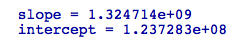
for param, value in std_params.iteritems():
print(str(param) + ' = %e' % value)
# Plot
data_plot = scatter_plot(OD_vs_CFU, markersize=20,
facecolor='red', axes_labels=['OD at 600nm', 'CFU/ml'])
fit_plot = plot(standard_curve(OD, std_params[slope],
std_params[intercept]), (OD, 0, 1.2))
show(data_plot+fit_plot)The results are as follows:
We introduced some new concepts in this example. On the first line, the statement import numpy allows us to access functions and classes from a module called NumPy. NumPy is based upon a fast, efficient array class, which we will use to store our data. We created a NumPy array and hard-coded the data values for OD, and created another array to store values of concentration (in practice, we would read these values from a file) We then defined a Python function called
standard_curve, which we will use to convert optical density values to concentrations. We used the
find_fit function to fit the slope and intercept parameters to the experimental data points. Finally, we plotted the data points with the scatter_plot function and the plotted the fitted line with the plot function. Note that we had to use a function called
zip to combine the two NumPy arrays into a single list of points before we could plot them with scatter_plot. We'll learn all about Python functions in Chapter 4, and Chapter 8 will explain more about fitting routines and other numerical methods in Sage.