

Now, let's fit a growth model to this data. The model we will use is based on the Gompertz function, and it has four parameters:
var('t, max_rate, lag_time, y_max, y0')
def gompertz(t, max_rate, lag_time, y_max, y0):
"""Define a growth model based upon the Gompertz growth curve"""
return y0 + (y_max - y0) * numpy.exp(-numpy.exp(1.0 +
max_rate * numpy.exp(1) * (lag_time - t) / (y_max - y0)))
# Estimated parameter values for initial guess
max_rate_est = (1.4e9 - 5e8)/200.0
lag_time_est = 100
y_max_est = 1.7e9
y0_est = 2e8
gompertz_params = find_fit(exp_data, gompertz,
parameters=[max_rate, lag_time, y_max, y0],
variables=[t],
initial_guess=[max_rate_est, lag_time_est, y_max_est, y0_est],
solution_dict = True)
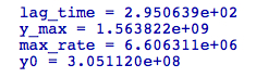
for param,value in gompertz_params.iteritems():
print(str(param) + ' = %e' % value)The fitted parameter values are displayed:
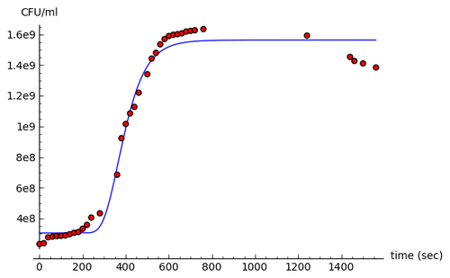
Finally, let's plot the fitted model and the experimental data points on the same axes:
gompertz_model_plot = plot(gompertz(t, gompertz_params[max_rate],
    gompertz_params[lag_time], gompertz_params[y_max],
    gompertz_params[y0]), (t, 0, sample_times.max()))

show(gompertz_model_plot + data_plot)
The plot looks like this:
We defined another Python function called gompertz
to model the growth of bacteria in the presence of limited resources. Based on the data plot from the previous example, we estimated values for the parameters of the model to use an initial guess for the fitting routine. We used the find_fit function again to fit the model to the experimental data, and displayed the fitted values. Finally, we plotted the fitted model and the experimental data on the same axes.