The main task while creating a launch file for the gmapping process is to set the parameters for the slam_gmapping node and the move_base node. The slam_gmapping node is the core node inside the ROS Gmapping package. The slam_gmapping node subscribes the laser data (sensor_msgs/LaserScan) and the TF data, and publishes the occupancy grid map data as output (nav_msgs/OccupancyGrid). This node is highly configurable and we can fine tune the parameters to improve the mapping accuracy. The parameters are mentioned at http://wiki.ros.org/gmapping.

The next node we have to configure is the move_base node. The main parameters we need to configure are the global and local costmap parameters, the local planner, and the move_base parameters. The parameters list is very lengthy. We are representing these parameters in several YAML files. Each parameter is included in the param folder inside the diff_wheeled_robot_gazebo package.

The following is the gmapping.launch file used in this robot. The launch file is placed in the diff_wheeled_robot_gazebo/launch folder:

<launch> 
  <arg name="scan_topic" default="scan" /> 
 
<!-- Defining parameters for slam_gmapping node --> 
 
  <node pkg="gmapping" type="slam_gmapping" name="slam_gmapping" output="screen"> 
    <param name="base_frame" value="base_footprint"/> 
    <param name="odom_frame" value="odom"/> 
    <param name="map_update_interval" value="5.0"/> 
    <param name="maxUrange" value="6.0"/> 
    <param name="maxRange" value="8.0"/> 
    <param name="sigma" value="0.05"/> 
    <param name="kernelSize" value="1"/> 
    <param name="lstep" value="0.05"/> 
    <param name="astep" value="0.05"/> 
    <param name="iterations" value="5"/> 
    <param name="lsigma" value="0.075"/> 
    <param name="ogain" value="3.0"/> 
    <param name="lskip" value="0"/> 
    <param name="minimumScore" value="100"/> 
    <param name="srr" value="0.01"/> 
    <param name="srt" value="0.02"/> 
    <param name="str" value="0.01"/> 
    <param name="stt" value="0.02"/> 
    <param name="linearUpdate" value="0.5"/> 
    <param name="angularUpdate" value="0.436"/> 
    <param name="temporalUpdate" value="-1.0"/> 
    <param name="resampleThreshold" value="0.5"/> 
    <param name="particles" value="80"/> 
  
    <param name="xmin" value="-1.0"/> 
    <param name="ymin" value="-1.0"/> 
    <param name="xmax" value="1.0"/> 
    <param name="ymax" value="1.0"/> 
 
    <param name="delta" value="0.05"/> 
    <param name="llsamplerange" value="0.01"/> 
    <param name="llsamplestep" value="0.01"/> 
    <param name="lasamplerange" value="0.005"/> 
    <param name="lasamplestep" value="0.005"/> 
    <remap from="scan" to="$(arg scan_topic)"/> 
  </node> 
 
<!-- Defining parameters for move_base node --> 
 
  <node pkg="move_base" type="move_base" respawn="false" name="move_base" output="screen"> 
    <rosparam file="$(find diff_wheeled_robot_gazebo)/param/costmap_common_params.yaml" command="load" ns="global_costmap" /> 
    <rosparam file="$(find diff_wheeled_robot_gazebo)/param/costmap_common_params.yaml" command="load" ns="local_costmap" /> 
    <rosparam file="$(find diff_wheeled_robot_gazebo)/param/local_costmap_params.yaml" command="load" /> 
    <rosparam file="$(find diff_wheeled_robot_gazebo)/param/global_costmap_params.yaml" command="load" /> 
    <rosparam file="$(find diff_wheeled_robot_gazebo)/param/base_local_planner_params.yaml" command="load" /> 
    <rosparam file="$(find diff_wheeled_robot_gazebo)/param/dwa_local_planner_params.yaml" command="load" /> 
    <rosparam file="$(find diff_wheeled_robot_gazebo)/param/move_base_params.yaml" command="load" /> 
 
  </node> 
 
</launch> 

We can build the ROS package called diff_wheeled_robot_gazebo and can run the gmapping.launch file for building the map. The following are the commands to start with the mapping procedure.

Start the robot simulation by using the Willow Garage world:

$ roslaunch diff_wheeled_robot_gazebo diff_wheeled_gazebo_full.launch

Start the gmapping launch file with the following command:

$ roslaunch diff_wheeled_robot_gazebo gmapping.launch

If the gmapping launch file is working fine, we will get the following kind of output on the Terminal:

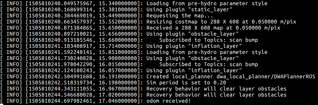
Figure 20: Terminal messages during gmapping

Start the keyboard teleoperation for manually navigating the robot around the environment. The robot can map its environment only if it covers the entire area:

$ roslaunch diff_wheeled_robot_control keyboard_teleop.launch

The current Gazebo view of the robot and the robot environment is shown next. The environment is with obstacles around the robot:

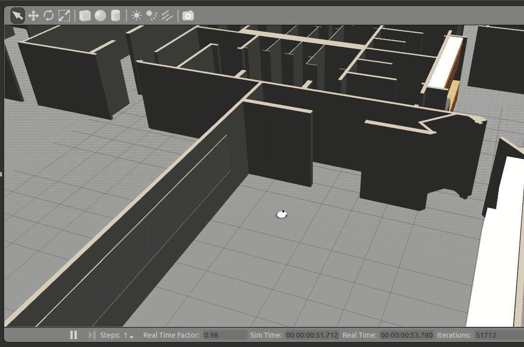
Figure 21: Simulation of the robot using the Willow Garage world

We can launch RViz and add a display type called Map and the topic name as /map.

We can start moving the robot inside the world by using key board teleoperation, and we can see a map building according to the environment. The following image shows the completed map of the environment shown in RViz:

Figure 22: Completed map of the room in RViz

We can save the built map using the following command. This command will listen to the map topic and save into the image. The map server package does this operation:

$ rosrun map_server map_saver -f willo

Here willo is the name of the map file. The map file is stored as two files: one is the YAML file, which contains the map metadata and the image name, and second is the image, which has the encoded data of the occupancy grid map. The following is the screenshot of the preceding command, running without any errors:

Figure 23: Terminal screenshot while saving a map

The saved encoded image of the map is shown next. If the robot gives accurate robot odometry data, we will get this kind of precise map similar to the environment. The accurate map improves the navigation accuracy through efficient path planning:

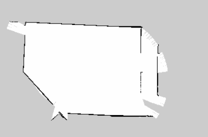
Figure 24: The saved map

The next procedure is to localize and navigate in this static map.

The ROS amcl package provides nodes for localizing the robot on a static map. The amcl node subscribes the laser scan data, laser scan based maps, and the TF information from the robot. The amcl node estimates the pose of the robot on the map and publishes its estimated position with respect to the map.

If we create a static map from the laser scan data, the robot can autonomously navigate from any pose of the map using amcl and the move_base nodes. The first step is to create a launch file for starting the amcl node. The amcl node is highly customizable; we can configure it with a lot of parameters. The list of parameters are available at the ROS package site (http://wiki.ros.org/amcl).

A typical amcl launch file is given next. The amcl node is configured inside the amcl.launch.xml file, which is in the diff_wheeled_robot_gazebo/launch/include package. The move_base node is also configured separately in the move_base.launch.xml file. The map file we created in the gmapping process is loaded here, using the map_server node:

<launch> 
 
  <!-- Map server --> 
  <arg name="map_file" default="$(find diff_wheeled_robot_gazebo)/maps/test1.yaml"/> 
  <node name="map_server" pkg="map_server" type="map_server" args="$(arg map_file)" /> 
 
 
  <include file="$(find diff_wheeled_robot_gazebo)/launch/includes/amcl.launch.xml"> 
 
    <arg name="initial_pose_x" value="0"/> 
    <arg name="initial_pose_y" value="0"/> 
    <arg name="initial_pose_a" value="0"/> 
 
  </include> 
 
  <include file="$(find diff_wheeled_robot_gazebo)/launch/includes/move_base.launch.xml"/> 
 
</launch> 

The following is the code snippet of amcl.launch.xml. This file is a bit lengthy, as we have to configure a lot of parameters for the amcl node:

<launch> 
  <arg name="use_map_topic"  default="false"/> 
  <arg name="scan_topic"     default="scan"/> 
  <arg name="initial_pose_x" default="0.0"/> 
  <arg name="initial_pose_y" default="0.0"/> 
  <arg name="initial_pose_a" default="0.0"/> 
 
  <node pkg="amcl" type="amcl" name="amcl"> 
    <param name="use_map_topic"             value="$(arg use_map_topic)"/> 
    <!-- Publish scans from best pose at a max of 10 Hz --> 
    <param name="odom_model_type"           value="diff"/> 
    <param name="odom_alpha5"               value="0.1"/> 
    <param name="gui_publish_rate"          value="10.0"/> 
    <param name="laser_max_beams"             value="60"/> 
    <param name="laser_max_range"           value="12.0"/> 

After creating this launch file, we can start the amcl node, using the following procedure:

Start the simulation of the robot in Gazebo:

$ roslaunch diff_wheeled_robot_gazebo diff_wheeled_gazebo_full.launch 

Start the amcl launch file, using the following command:

$ roslaunch diff_wheeled_robot_gazebo amcl.launch

If the amcl launch file is correctly loaded, the Terminal shows the following message:

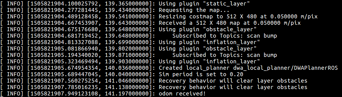
Figure 25: Terminal screenshot while executing amcl

If amcl is working fine, we can start commanding the robot to go into a position on the map using RViz, as shown in the following figure. In the figure, the arrow indicates the goal position. We have to enable LaserScan, Map, and Path visualizing plugins in RViz for viewing the laser scan, the global/local costmap, and the global/local paths. Using the 2D NavGoal button in RViz, we can command the robot to go to a desired position.

The robot will plan a path to that point and give velocity commands to the robot controller to reach that point:

Figure 26: Autonomous navigation using amcl and the map

In the preceding image, we can see that we have placed a random obstacle in the robot's path, and that the robot has planned a path to avoid the obstacle.

We can view the amcl particle cloud around the robot by adding a Pose Array on RViz and the topic is /particle_cloud. The following image shows the amcl particle around the robot:

Figure 27: The amcl particle cloud and odometry