Book Image

Julia Programming Projects

By : Adrian Salceanu
Book Image

Julia Programming Projects

By: Adrian Salceanu

Overview of this book

Julia is a new programming language that offers a unique combination of performance and productivity. Its powerful features, friendly syntax, and speed are attracting a growing number of adopters from Python, R, and Matlab, effectively raising the bar for modern general and scientific computing. After six years in the making, Julia has reached version 1.0. Now is the perfect time to learn it, due to its large-scale adoption across a wide range of domains, including fintech, biotech, education, and AI. Beginning with an introduction to the language, Julia Programming Projects goes on to illustrate how to analyze the Iris dataset using DataFrames. You will explore functions and the type system, methods, and multiple dispatch while building a web scraper and a web app. Next, you'll delve into machine learning, where you'll build a books recommender system. You will also see how to apply unsupervised machine learning to perform clustering on the San Francisco business database. After metaprogramming, the final chapters will discuss dates and time, time series analysis, visualization, and forecasting. We'll close with package development, documenting, testing and benchmarking. By the end of the book, you will have gained the practical knowledge to build real-world applications in Julia.
Table of Contents (19 chapters)
Title Page
Copyright and Credits
Dedication
About Packt
Contributors
Preface
Index

Time series decomposition


We can thus say that any value in a time series can be represented through a function of the four components we discussed earlier—trend, seasonality, error, and cycle. The relationship between the four components can be either additive or multiplicative.

The additive model is used when the seasonal variation stays about the same across time. The trend may be upward or downward, but the seasonality stays more or less the same. A plot of such data will look very similar to this:

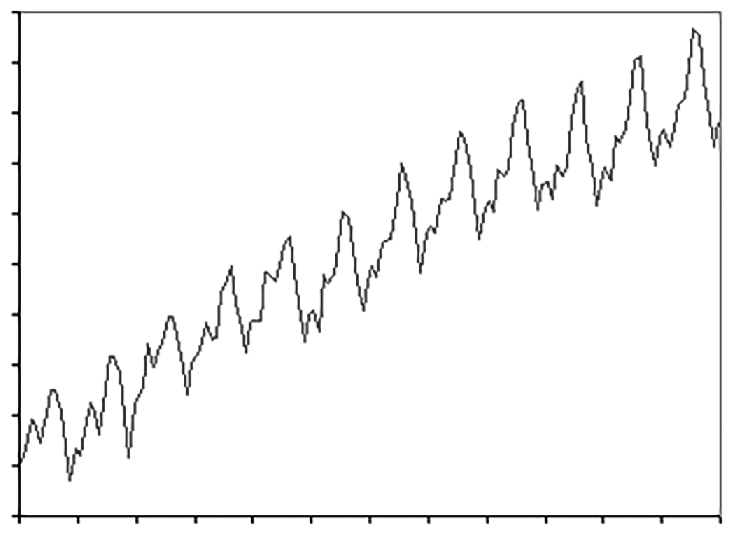
If we draw two imaginary lines between the yearly maximums and the yearly minimums, the lines will be pretty much parallel.

For an additive time series model, the four components are summed up to produce the values in the series. Thus, a time series Y can be decomposed into Y = Trend + Cycle + Seasonality + Noise.

A multiplicative model should be used with a time series where the seasonal variability increases over time. For example, a typical multiplicative time series is represented by the international...