


We've used some of R's built-in datasets so far in this book, but most of the time, data scientists will have to import and export data that comes from external sources in and out of R. Data can come and go in many different forms, and while we'll not cover them all here, we'll touch on some of the most common forms.
Data import and export are truly one subsection in R, because most of the time, the functions are opposites: for example, read.csv() takes in the character string name of a .csv file, and you save the output as a dataset in your environment, while write.csv() takes in the name of the dataset in your environment and the character string name of a file to write to.
There are built-in functions in R for the data import and export of many common file types, such as read.table() for .txt files, read.csv() for .csv files, and read.delim() for other types of delimited files (such as tab or | delimited, where | is the pipe operator appropriated as a separator). For pretty much any other file type, you have to use a package, usually one written for the import of that particular file type. Common data import packages for other types of data, such as SAS, Excel, SPSS, or Stata data, include the packages readr, haven, xlsx, Hmisc, and foreign:
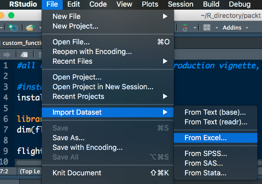
RStudio also has point and click methods for importing data. If you navigate to File | Import Dataset, you'll see that you have six options:
- From text (base)
- From text (readr)
- From Excel
- From SPSS
- From SAS
- From Stata
These options call the required packages and functions that are necessary to input data of that type into R. The packages and functions are listed in order, as follows:
- base::read.table()
- readr::read_* functions
- xlsx::read_excel()
- haven::read_sav()
- haven::read_sas()
- haven::read_dta()
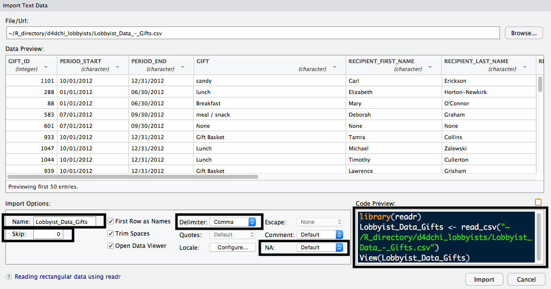
One advantage of loading data using one of these functions is that you can see the Import Text Data window. This window allows you to toggle different options, such as what to Name the dataset once it's imported, which Delimiter is used, how many rows to Skip, what value to use for missing data, and more. There's also a Code Preview, which allows you to see what the code will look like when you import your data. The following screenshot displays this:
To use most of these functions, you must follow these basic steps:
- Figure out what type of data you're dealing with—is it a CSV? Is it from SAS? and so on.
- Find the appropriate function to import that type of data.
- The first (and sometimes only argument) to the function is a character string indicating where that data is located on your computer.
- If applicable, tweak the settings of the appropriate function, such as indicating the separator with sep or setting stringAsFactors.
Synthetic data means it was created for the purposes of this exercise and is not a dataset collected from an experiment. The dataset is saved in three formats:
- Text-delimited .txt file
- comma-separated values .csv file
- Microsof Excel worksheet .xlsx file
We'll be downloading all three of these directly from GitHub and importing them into RStudio. To do so, we'll need to use the URL, as a character string, as the first argument to all of the functions we'll use to import data.
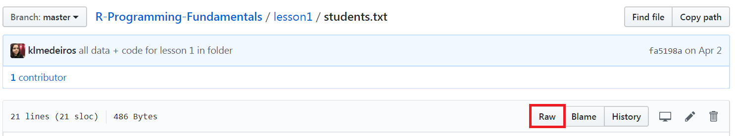
We can import data directly from GitHub by using the read.table() function. If we input the URL where the dataset is stored, the function will download it for you, as shown in the following example:
students_text <- read.table("https://raw.githubusercontent.com/TrainingByPackt/R-Programming-Fundamentals/master/lesson1/students.txt")
While this code will read in the table, if we open and examine it, we will notice that the variable names are currently the first row of the dataset. To find the options for read.table(), we can use the following command:
?read.table
Reading the documentation, it says that the default value for the header argument is FALSE. If we set it to TRUE, read.table() will know that our table contains—as the first row—the variable names, and they should be read in as names. Here is the example:
students_text <- read.table("https://raw.githubusercontent.com/TrainingByPackt/-Programming-Fundamentals/master/lesson1/students.txt",header = TRUE)
The data has now been imported correctly, with the variable names in the correct place.
We may want to convert the Height_inches variable to centimeters and the Weight_ lbs variable to kilograms. We can do so with the following code:
students_text$Height_cm <- (students_text$Height_inches * 2.54)
students_text$Weight_kg <- (students_text$Weight_lbs / 0.453592)
Since we've added these two variables, it may now be necessary to export the table out of R, perhaps to email it to a colleague for their use or to re-upload it on GitHub. The opposite of read.table() is write.table(). Take a look at the following example:
write.table(students_text, "students_text_out.txt")
This will write out the students_text dataset we're using in R to a file called students_text_out in our working directory folder on our machine.
There are additional options for read.table() that we could use as well. We can actually import a .csv file this way by setting the sep argument equal to a comma. We can skip rows with skip = some number, and add our own row names or column names by passing in a vector of either of those to the row.names or col.names argument.
Most of the other data import and export functions in R work much like read. table() and write.table(). Let's import the students' data from the .csv format, which can be done in three different ways, using read.table(), read.csv(), and read_csv().
- Import the students.csv file from GitHub using read.table(). Save it as a dataset called students_csv1, using the following code:
students_csv1 <-read.table("https://raw.githubusercontent.com/TrainingByPackt/R-Programming-Fundamentals/master/lesson1/students.csv", header = TRUE, sep = ",")
- Import students.csv using read.csv(), which works very similar to read. table():
students_csv2 <- read.csv("https://raw.githubusercontent.com/TrainingByPackt/R-Programming-Fundamentals/master/lesson1/students.csv")
- Download the readr package:
install.packages("readr")
- Load the readr package:
library(readr)
- Import students.csv using read_csv():
students_csv3 <- read_csv("https://raw.githubusercontent.com/TrainingByPackt/R-Programming-Fundamentals/master/lesson1/students.csv")
- Examine students_csv2 and students_csv3 with str():
str(students_csv2)
str(students_csv3)
Output:
The output for the str(students_csv2) function is as follows:
'data.frame': 20 obs. of 5 variables:
$ Height_inches: int 65 55 60 61 62 66 69 54 57 58 …
$ Weight_lbs: int 120 135 166 154 189 200 250 122 101 178 …
$ EyeColor: Factor w/ 4 levels "Blue","Brown",…: 1 2 4 2 3 3 1 1 1 2 …
$ HairColor: Factor w/ 4 levels "Black","Blond",…: 3 2 1 3 2 4 4 3 3 1 …
$ USMensShoeSize: int 9 5 6 7 8 9 10 5 6 4 …
The output for the str(students_csv3) function is as follows:
Classes 'tbl_df', 'tbl' and 'data.frame': 20 obs. of 5 variables:
$ Height_inches : int 65 55 60 61 62 66 69 54 57 58 …
$ Weight_lbs : int 120 135 166 154 189 200 250 122 101 178 …
$ EyeColor : chr "Blue" "Brown" "Hazel" "Brown" … $ HairColor : chr "Brown" "Blond" "Black" "Brown" …
$ USMensShoeSize: int 9 5 6 7 8 9 10 5 6 4 …
A few notes about the three different ways we read in the .csv file in the exercise are as follows:
- read.table(), with header = TRUE and sep = "," reads the data in correctly
- For read.csv(), the header argument is TRUE by default, so we don't have to specify it:
- If we view the dataset, using str(students_csv2), we can see that the HairColor and EyeColor variables got read in as factor variables by default
- This is because the stringsAsFactors option is TRUE by default for read.csv()
- For read_csv() in the readr package, the opposite is true about the default stringsAsFactors value; it is now FALSE:
- Therefore, HairColor and EyeColor are read in as character variables. You can verify this with str(students_csv3)
- If we wanted factor variables, would have to change the variables ourselves after import or set stringsAsFactors = TRUE to automatically import all character variables as factors, as in read.csv()


