In this section, we will dive into three crucial topics of mathematics that are used heavily in quantum computation – coordinate systems, complex numbers, and probability. Coordinate systems are useful for the graphical representation of quantum states and to describe mathematical calculations in a visual format. After a fundamental understanding of coordinate systems, we will move on to complex numbers and look at their relationship with coordinate systems. You will see the simplicity of calculations carried out using the complex plane. Finally, we will learn about some fundamental probability theory concepts that are useful to quantum computing. Let's start with coordinate systems.
Introducing coordinate systems
In this section, you will learn about visualizing quantum states, which are just vectors in a mathematical sense. This will be useful for visualizing the geometry of quantum states and the various operations that you have already learned about in the previous sections. We will start with 2D coordinate systems and then move on to 3D coordinates before learning about the polar coordinate system.
2D Cartesian coordinate systems
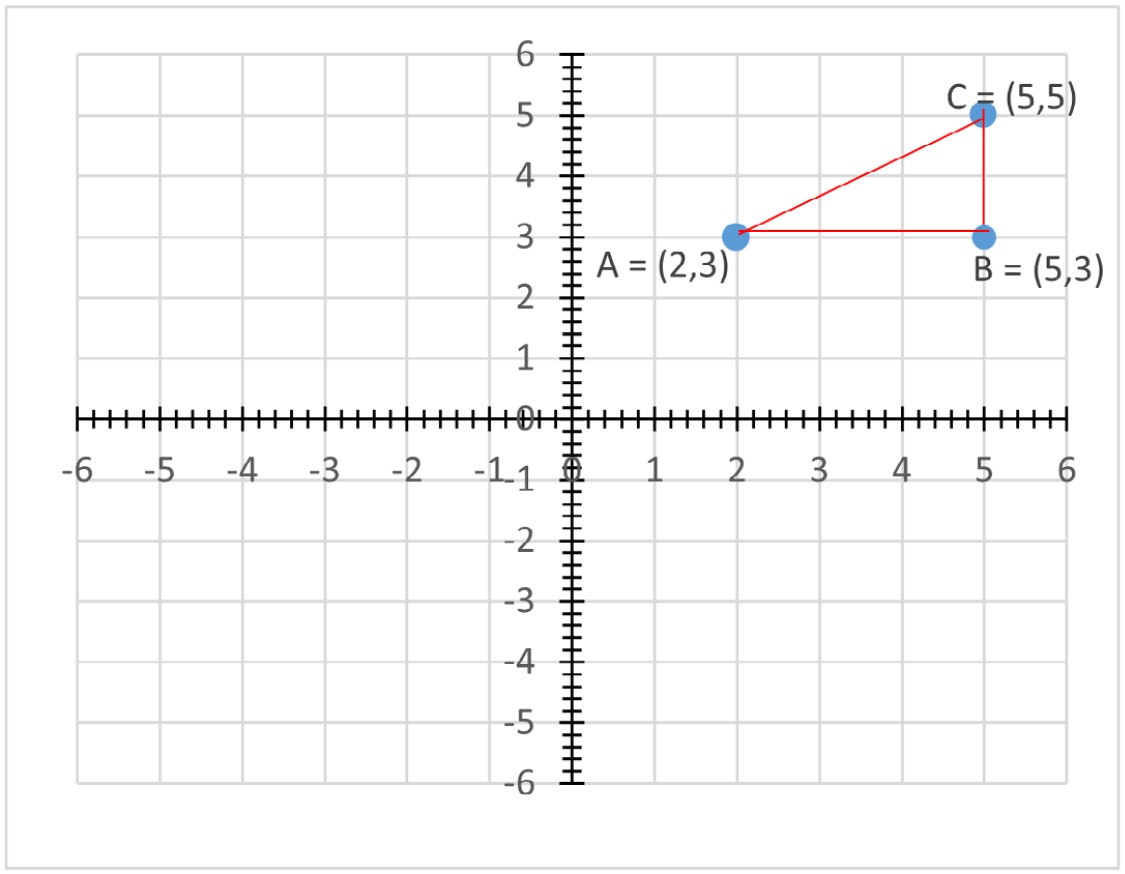
Cartesian coordinates are one of the most useful graphical ways of visualizing 2D and 3D planes. Figure 1.1 shows the 2D coordinate system and displays the coordinates and vectors present in the space:
Figure 1.1 – A 2D Cartesian coordinate system
The coordinates in the Cartesian plane (Euclidean space) are denoted as (x,y), where the horizontal line is the x-axis and the vertical line is the y-axis; for example, in the preceding figure, three coordinates are represented as A = (2,3), B = (5,3), and C = (5,5). The point O = (0,0) is the origin. Using these coordinate values and the Pythagoras theorem for right triangles, the length AC can be calculated as  . The distances in the Cartesian plane are called the Euclidean distance. This can be used to plot various kinds of functions, such as polynomial curves, circles, hyperbola, and exponentials. Cartesian coordinates can also be written in column vector form as
  .
.
We will now move on to 3D coordinate systems and understanding their usefulness.
3D Cartesian coordinate systems
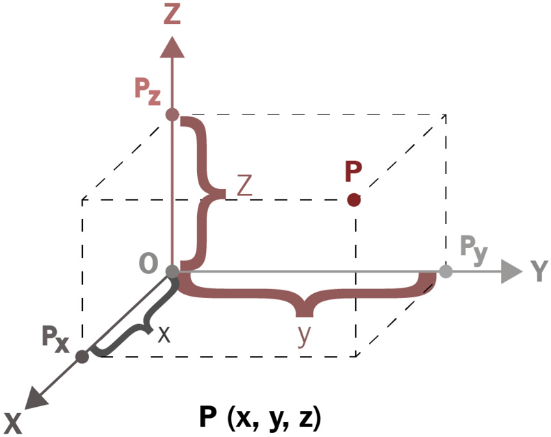
In a 3D Cartesian system, we have 3 axes – the x-axis, the y-axis, and the z-axis. Often, we have to use 3D representations of vectors to understand the higher-dimensional aspect of quantum computing. Figure 1.2 shows the 3D coordinate system, and this coordinate system turns out to be very useful for understanding and visualizing higher-dimensional computations:
Figure 1.2 – A 3D Cartesian coordinates system
The coordinates can be denoted as (x,y,z). In this case, the x-axis is the tilted axis, the y-axis is the horizontal axis, and the z-axis represents the height or vertical axis. The mathematical calculations used for 2D systems can also be utilized for 3D systems. This 3D coordinate system will be very useful when we discuss Bloch sphere representations of qubits in Chapter 2, Quantum Bits, Quantum Measurements, and Quantum Logic Gates.
Next, we will introduce the polar coordinates system and discuss the conversion of coordinates between Cartesian and polar coordinate systems.
Converting Cartesian systems to polar coordinate systems
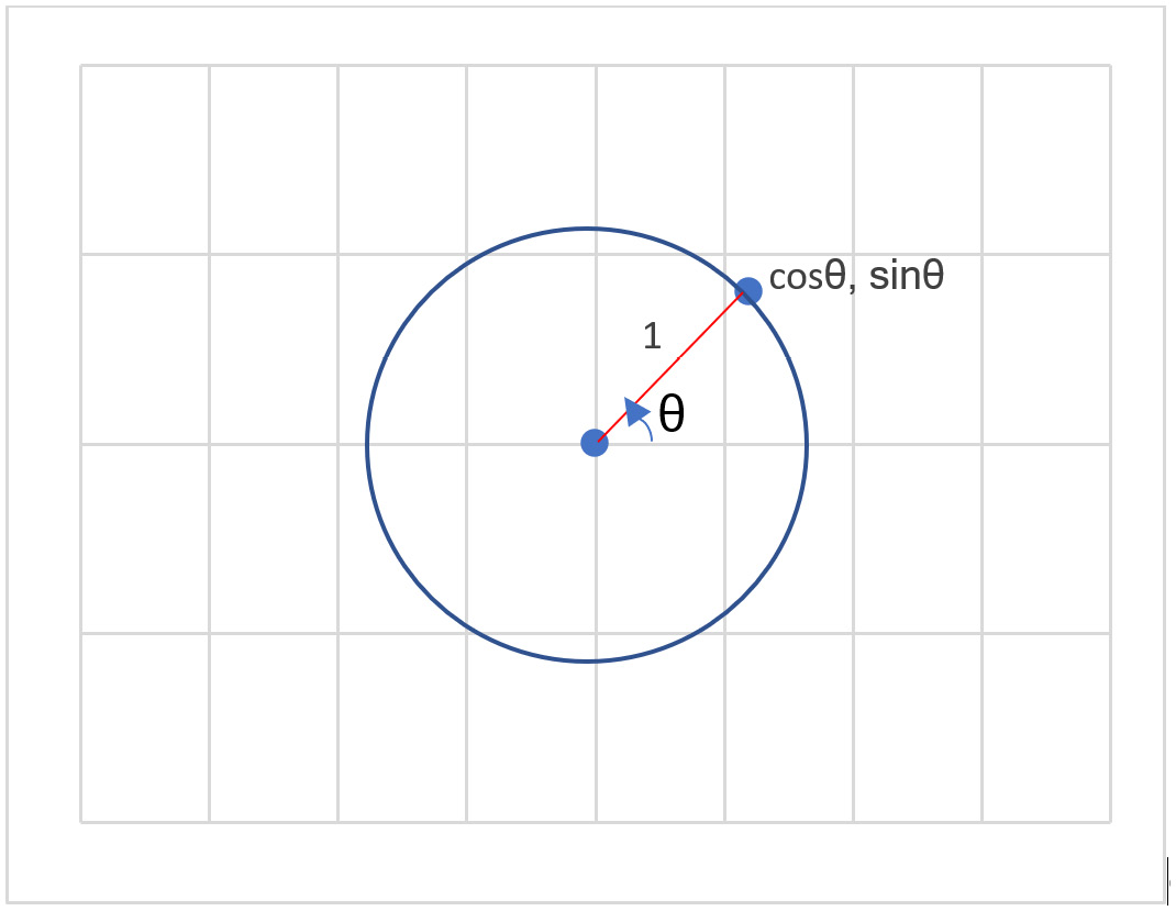
For simple calculations and complex numbers (covered in the next section), it is useful to convert Cartesian coordinates to polar coordinates, which involves using trigonometric functions. Polar coordinates are easily represented using a unit circle given in a 2D Cartesian plane. Figure 1.3 shows the polar coordinate system:
Figure 1.3 – Polar coordinate system
In a polar coordinate system, the (x,y) coordinates are represented as  , where r is the radius and is given as
  and
and  in degrees. To convert degrees into radians, multiply the degree value by
  . To convert radians back into degrees, multiply by
  . If you want to convert from polar to Cartesian, then you can use
  and
and  . The polar representation that we learned about will be very useful for the calculations related to complex numbers.
Complex numbers and the complex plane
Jerome Cardan introduced the concept of complex numbers when it was found that while solving the roots of a quadratic polynomial, the square roots of negative numbers were encountered, which were not covered by real numbers. Due to this, the imaginary unit  was introduced. This helped to write numbers such as
A complex number consists of real and imaginary parts. It is defined as follows:

Here, a and b are real numbers. In this, a is the real component and i b is the imaginary component, where b is the imaginary coefficient. Again, a complex number can be represented as a vector. In vector form, it z 
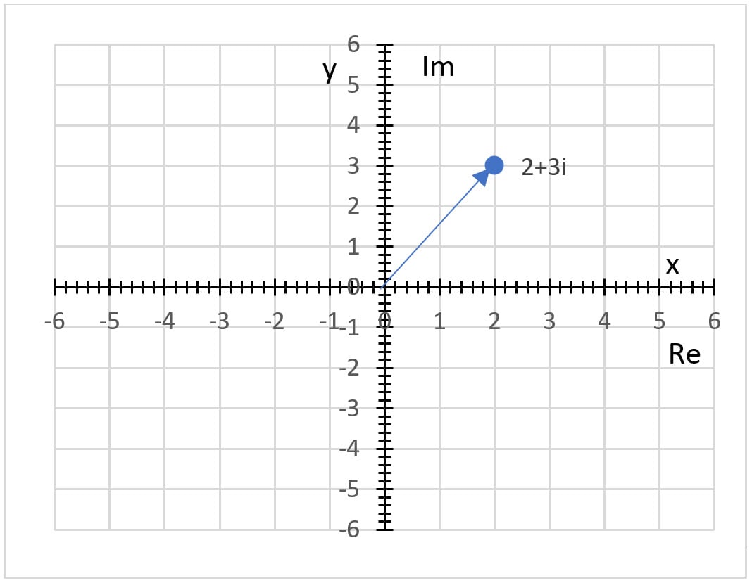
 . In Figure 1.4, the complex number
  is shown:
Figure 1.4 – The Cartesian plane representing complex numbers
In the preceding figure, you can see that the complex number  has been represented in a Cartesian plane, where the x-axis denotes the real component and the y-axis denotes the imaginary component, more specifically, the imaginary coefficient, which is a real number.
Performing arithmetic operations on complex numbers is fairly intuitive and usually follows the normal algebraic rules.
For example, let's see the addition of two complex numbers:

The addition of complex numbers is commutative and associative, as follows:
- Commutative:
 , for example,
- Associative:
 , for example,
Subtraction is similar to addition. Let's see the multiplication of two complex numbers:

Similar to addition, multiplication has commutative and associative properties, along with another property called the distributive property. This is shown as follows:
- Commutative:
 , for example,
- Associative:
 , for example,
- Distributive:
 , for example,
The complex conjugate of a complex number is given as follows:

The complex conjugate shows us the reflection of the complex number in another part of the axis provided in the complex plane.
The modulus of a complex number is very similar to calculating the magnitude of a vector and is given as follows:

We saw the polar coordinate system in the previous section and discussed how it is useful in the case of complex number representation. We will now look at using the polar coordinate system for complex number representation, which is a very important method to consider.
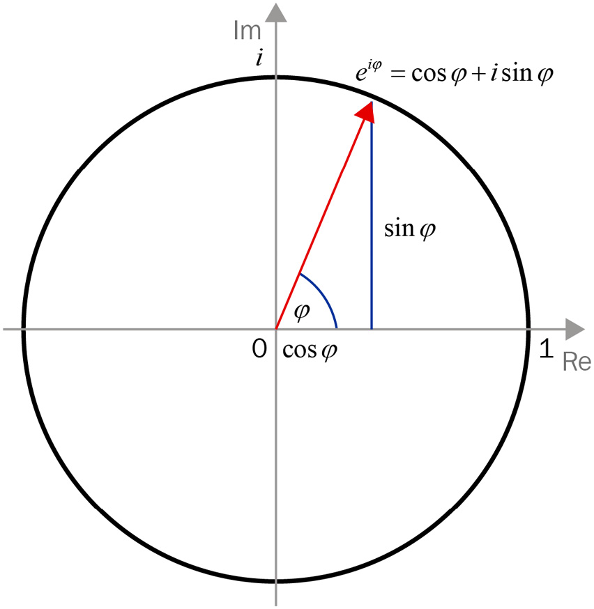
The main formula that connects polar coordinates with the complex plane is known as Euler's formula. The complex plane can be defined as a geometric visualization of the complex numbers in a 2D coordinate system, where the x-axis becomes the real part and the y-axis becomes the imaginary part. This is also known as the z-plane. Figure 1.5 shows the complex plane along with the Euler's relation, where  (phi) is the angle:
Figure 1.5 – Euler's formula representation using a unit circle
Euler's formula is given as follows:


This formula helps connect the trigonometric relations with the complex exponentials. This helps us to represent a complex number in a polar representation. Let's define the complex number as follows:

Here, putting  will give z as follows:
 given as
  and
and  in degrees.
If you calculate  , you will see that it is always 1, and you can verify it yourself. It will require the usage of one of the most common trigonometric identities. Euler's identity is given as
  and is usually a good thing to know!
It is important to be familiar with some identities that make our mathematical calculations easier for the case of complex numbers. Two identities that are useful are these:
 and
and 
These identities are essentially representations of common trigonometric functions in terms of their complex exponentials.
The complex conjugate of  is
is  . The complex exponential form makes the calculations a lot easier.
Let's now dive into the topic of probability and learn about its significance in the field of quantum computing.
Probability
The concept of probability theory has always found significance in almost every area of science and technology, and quantum computing is no exception. Probability is a useful tool for dealing with the inherent randomness of real-life situations. In this section, we will dive into the basics of probability, random variables, and the usefulness of probability in quantum computing. Let's start with the definition of probability and its basic axioms.
Probability basics and axioms
Probability, as you might have guessed, is a branch of mathematics that deals with the likelihood or chance of events occurring. It is helpful in representing the likelihood of events happening in a system in terms of mathematical language. Girolamo Cardan wrote a book called Book on Games of Chance that introduced the first systematic treatment of the theory of probability.
Today, the applications of probability are huge in number because probabilistic techniques are used to predict the outcomes of various situations. It is used in games, weather forecasting, sports predictions, machine learning methods, reinforcement learning in artificial intelligence, deep learning, and quantum mechanics and physics for quantum measurement theory.
In quantum measurement theory, we check and calculate the probabilities of a quantum state being collapsed to a certain state. This is where the tools of probability theory are very useful. To make a probabilistic model of an unknown situation, two important things need to be considered: sample space and the law of probability.
Let's understand sample space first. A sample space is a set or collection of all the possible outcomes of a particular event. It is usually denoted by  (pronounced as omega). For example, for an experiment of flipping a coin, we have a total of two possible outcomes, which are heads (H) and tails (T). So, the sample
  .
.
The law of probability assigns a numerical value (non-negative) to a particular event that represents the likelihood of that event occurring out of all the possible events. This is usually given as follows:

For example, the probability that tails can occur when we flip a coin is as follows:
P(T) = 
Now we will look at some fundamental axioms of probability that are necessary for understanding the law of probability:
- Probability can't be negative: This means that the probability of events from the sample space must be greater than or equal to zero.
 for every A.
- Probability addition: For two disjointed events A and B, their probability of union is given by the sum of their individual probabilities.
 when P(A) and P(B) are independent events. If events are not independent, then
  .
.
- The sum of all probabilities must be 1: The probability of the entire sample space must be equal to 1. P(
 ) = 1.
It is important to mention that  , which is a complementary probability, and
  . Also, the probability values of a certain event A from the sample space must be
  so that the sum of all the probabilities of events present in the sample space adds up to 1. We observed that probabilities often have a numerical value, but many variables in the real world do not possess numerical values, so now we will discuss this issue in the next section by introducing random variables.
Discrete random variables and probability mass functions
Many times in the real world, the outcome of the events that we measure may not be numerical in nature. In those cases, random variables come to our rescue.
Random variables entail a mapping process that assigns a numerical value to the outcome of the events happening in a sample space. So, the random variable works as a function by taking outcomes from the sample space and giving them a numerical value taken in a real number line. In our case, we will be discussing discrete random variables.
Discrete random variables can be associated with a probability distribution, which is known as the Probability Mass Function (PMF). The PMF provides the probability of each of the numerical values that a discrete random variable can take. The sum of elements of the PMF always adds up to 1.
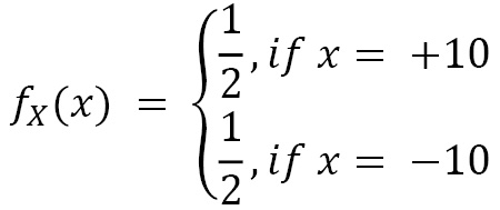
Let's consider a situation where a coin is flipped and every time heads comes up, you win $10, and every time tails comes up, you lose $10.
In random variable notation, this can be described as follows:

To describe the PMF for this coin flipping experiment, we have this:
Randomness, as we have seen, is a very useful phenomenon and has a wide variety of applications. In practical coding implementation, we have pseudo-random number generators that generate numbers between 0 and 1, but the process of generation is not truly random. This process is called sampling. One of the most useful benefits of a quantum computer would be to generate truly random numbers.
We will now focus our attention on calculating the mean and variance when data is provided to us.
Expectation (mean value) and variance calculation
The expectation is simply the mean of a random variable. It is the weighted mean of all the possible values of a random variable. The weights used for the purpose of expectation calculation are in proportion to the probabilities of the outcome of events. From the perspective of the PMF, the expected value of the PMF denotes the center of gravity of that PMF distribution. This is like calculating a linear combination of outcomes where the weights are the probabilities. Mean is also known as the first moment in statistics.
The formula that is used to calculate the expectation is as follows:

As an example, for a 6-sided die toss, we have the probability of each side as  . Now, to calculate the expectation of this event, we need to multiply the probability by each of the numbered sides (the values of the outcomes), as shown here:

Variance is the measure of dispersion around the mean value. Intuitively, variance is about measuring the expected value of dispersion or the spread of the random variables from their mean value. Variance is also known as the second moment in statistics.
Therefore, the formula for variance becomes as follows:

Again, by considering the same 6-sided die example, we can calculate its variance as follows:

Essentially, variance defines the spread from the mean value, and in our case, the value is 2.92. In the next section, we will learn about the significance of the law of large numbers.
The law of large numbers
The law of large numbers states that the average or mean value of a large number of trials will be closer to the expected value and will tend to be closer and closer as the number of trials increases significantly.
In quantum computing, we perform measurements of probabilities of quantum states occurring after the quantum states are passed through a quantum circuit. This is done a number of times because the quantum computers that we have today are noisy and the quantum states that are prepared in the computer carry a lot of noise. So, to get accurate probability measurements, we run the measurements multiple times, and this is where the law of large numbers comes in. After a certain number of iterations of measurements, we start getting closer to the expected value, which is the ideal value.
With the conclusion of our discussion of probability, we also conclude our discussion of the essential mathematical concepts that are required for quantum computing. Let's now dive into the basics of algorithmic thinking and computer science that are essential for understanding quantum computing.


 Free Chapter