Low-level programming with C++

Initially, C++ was perceived as the successor of the C language; however, since then, it has evolved into something big, sometimes scary, and even untamable. With recent language updates, it now represents a complex beast that requires time and patience to tame. We will start this chapter by covering the basic constructs that almost every language supports, such as data types, conditional and loop statements, pointers, structs, and functions. We will look at those constructs from the perspective of a low-level systems programmer, curious about how even a simple instruction can be executed by the computer. A deep understanding of these basic constructs is mandatory to build a solid base for more advanced and abstract topics such as object-oriented programming (OOP).

Functions

Program execution starts with the main() function, which is the designated start of the program, as stated in the standard. A simple program outputting the Hello, World! message will look like this:

#include <iostream.h>
int main() {
    std::cout << "Hello, World!" << std::endl;
    return 0;
}

You may have encountered or used the arguments of the main() function in your passwords. It has two arguments, argc and argv, that allow strings to be passed from the environment. These are usually referred to as command-line arguments.

The names argc and argv are conventional and can be replaced with anything you want. The argc argument holds the number of command-line arguments passed to the main() function; the argv argument holds the necessary arguments (you can find the example code at https://github.com/PacktPublishing/Expert-C-2nd-edition/tree/main/Chapter%2001/2_argc_and_argv_usage.cpp).

For example, we can compile and run the preceding example with the following arguments:

$ my-program argument1 hello world --some-option

This will output the following to the screen:

The number of passed arguments is: 5
   Arguments are:
   argument1
   hello
   world
   --some-option

When you look at the number of arguments, you’ll notice that it is 5. The first argument is always the name of the program; that’s why we skipped it in this example by starting the loop from number 1.

Note

Rarely, you may see a widely supported but not standardized third argument, most commonly named envp. The type of envp is an array of char pointers and it holds the environment variables of the system.

The program can contain lots of functions, but the execution of the program always starts with the main() function, at least from the programmer’s perspective. Let’s try to compile the following code:

#include<iostream>
   void foo() {
   std::cout << "Risky foo" << std::endl;
}
// trying to call the foo() outside of the main() function
foo();
int main() {
     std::cout << "Calling main" << std::endl;
     return 0;
}

g++ raises an error on the foo(); call – that is, C++ requires a type specifier for all declarations. The call was parsed as a declaration rather than an instruction to execute. The way we tried to call a function before main() might seem silly for seasoned developers, so let’s try another way. What if we declare something that calls a function during its initialization? In the example at https://github.com/PacktPublishing/Expert-C-2nd-edition/tree/main/Chapter%2001/3_before_main.cpp, we defined a BeforeMain struct with a constructor printing a message, and then declared an object of the BeforeMain type in the global scope.

The example successfully compiles and the program outputs the following:

Constructing BeforeMain
Calling main()

What if we add a member function to BeforeMain and try to call it? See the following code to understand this:

struct BeforeMain {
 // constructor code omitted for brevity
   void test() {
       std::cout << "test function" << std::endl;
   }
};
BeforeMain b;
b.test(); // compiler error
int main() {
     // code omitted for brevity
}

The call to test() won’t be successful. So, we cannot call a function before main() but we can declare variables – objects that would be initialized by default. So, there is something that performs initialization before main() is called. It turns out that the main() function is not the true starting point of a program. The actual starting function of the program prepares the environment – that is, it collects the arguments that were passed to the program and then calls the main() function. This is required because C++ supports global and static objects that need to be initialized before the program begins, which means before the main() function is called. In the Linux world, this function is referred to as __libc_start_main. The compiler augments the generated code with the call of __libc_start_main, which, in turn, may or may not call other initialization functions before the main() function gets called. Going abstract, just imagine that the preceding code will be altered to something similar to the following:

void __libc_start_main() {
    BeforeMain b;
    main();
}
__libc_start_main(); // call the entry point

Recursion

Another special property of main() is that it cannot be called recursively. From the perspective of the OS, the main() function is the entry point of the program, so calling it again would mean starting everything over; therefore, it is prohibited. However, calling a function recursive just because it calls itself is partially correct. For example, the print_number() function calls itself and never stops:

void print_number(int num) {
    std::cout << num << std::endl;
    print_number(num + 1); // recursive call
}

Calling the print_number(1) function will output numbers 1, 2, 3, and so on. This is more like a function that calls itself infinitely rather than a correct recursive function. We should add a couple more properties to make the print_number() function a useful recursive one. First of all, the recursive function must have a base case, a scenario when a further function calls stop, which means the recursion stops propagating. We can make such a scenario for the print_number() function if, for example, we want to print numbers up to 100:

void print_number(int num) {
     if (num > 100) return; // base case
     std::cout << num << std::endl;
     print_number(num + 1); // recursive call
}

There is one more property for a function to be recursive: solving smaller problems that will eventually lead to the base case. In the preceding example, we already had this by solving a smaller problem for the function – that is, by printing one number. After printing one number, we move to the next small problem: printing the next number. Finally, we get to the base case and we are done. There isn’t any magic in a function calling itself; think of it as a function calling a different function with the same implementation. What’s interesting is how a recursive function affects the program’s execution overall. Let’s take a look at a simple example of calling a function from another function at https://github.com/PacktPublishing/Expert-C-2nd-edition/tree/main/Chapter%2001/5_calculate.cpp.

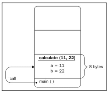
When a function is called, memory space is allocated for its arguments and local variables. The program starts with the main() function, which in this example simply calls the calculate() function by passing the 11 and 22 literal values. Control jumps to the calculate() function and the main() function is kind of on hold; it waits until the calculate() function returns to continue its execution. The calculate() function has two arguments, a and b; although we named sum(), max(), and calculate() differently, we could use the same names in all the functions. Memory space is allocated for these two arguments. Let’s suppose that an int takes 4 bytes of memory, so a minimum of 8 bytes are required for the calculate() function to be executed successfully. After allocating 8 bytes, 11 and 22 should be copied to the corresponding locations (see the following diagram for details):

Figure 1.4: The calculate() function call

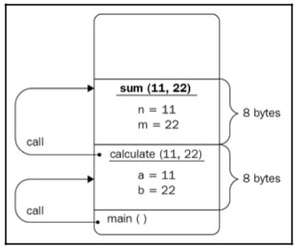
The calculate() function calls the sum() and max() functions and passes its argument values to them. Correspondingly, it waits for both functions to be executed sequentially to form the value to return to main(). The sum() and max() functions are not called simultaneously. First, sum() is called, which leads to the values of the a and b variables being copied from the locations that were allocated for the arguments of sum(), named n and m, which again take 8 bytes in total. Take a look at the following diagram to understand this better:

Figure 1.5: The calculate() function calls the sum() function

Their sum is calculated and returned. After the function is done and it returns a value, the memory space is freed. This means that the n and m variables are not accessible anymore and their locations can be reused.

Important note

We aren’t considering temporary variables at this point. We will revisit this example later to show the hidden details of function execution, including temporary variables and how to avoid them as much as possible.

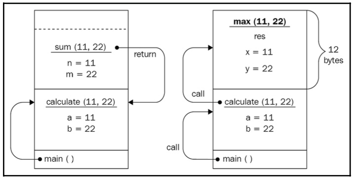
After sum() has returned a value, the max() function is called. It follows the same logic: memory is allocated to the x and y arguments, as well as to the res variable. We intentionally store the result of the ternary operator, (?:), in the res variable to make the max() function allocate more space for this example. So, 12 bytes are allocated to the max() function in total. At this point, the x main() function is still on hold and waits for calculate(), which, in turn, is on hold and waits for the max() function to complete (see the following diagram for details):

Figure 1.6: The max() function call after the sum() function is returned

When max() is done, the memory that’s allocated to it is freed and its return value is used by calculate() to form a value to return. Similarly, when calculate() returns, the memory is freed and the main() function’s local variable result will contain the value returned by calculate().

The main() function then finishes its work and the program exits – that is, the OS frees the memory allocated for the program and can reuse it later for other programs. The described process of allocating and freeing memory (deallocating it) for functions is done using a concept called a stack.

Note

A stack is a data structure adapter, which has rules to insert and access the data inside of it. In the context of function calls, the stack usually means a memory segment provided to the program that automatically manages itself while following the rules of the stack data structure adapter. We will discuss this in more detail later in this chapter.

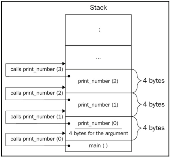
Going back to recursion, when the function calls itself, memory should be allocated to the newly called function’s arguments and local variables (if any). The function calls itself again, which means the stack will continue to grow (to provide space for the new functions). It doesn’t matter that we call the same function; from the stack’s perspective, each new call is a call to a completely different function, so it allocates space for it with a serious look on its face while whistling its favorite song. Take a look at the following diagram:

Figure 1.7: Illustration of a recursive function call inside the stack

The first call of the recursive function is on hold and waits for the second call of the same function, which, in turn, is on hold, and waits for the third call to finish and return a value, which, in turn, is on hold, and so on. If there is a bug in the function or the recursion base is difficult to reach, sooner or later, the stack will overgrow, which will lead to a program crash. This is known as stack overflow.

Though recursion provides more elegant solutions to a problem, try to avoid recursion in your programs and use the iterative approach (loops). In mission-critical system development guidelines such as the navigation system of a Mars rover, using recursion is completely prohibited.

Data and memory

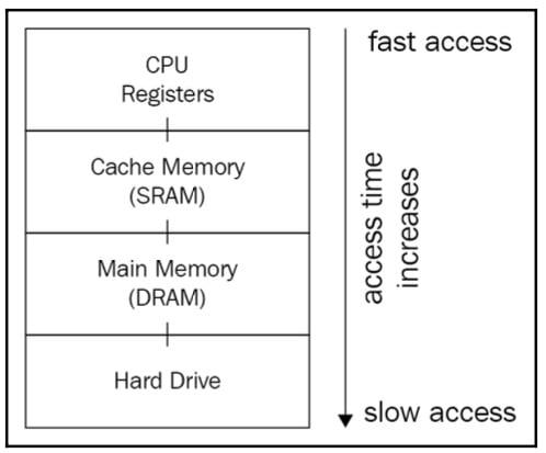
When we refer to computer memory, we consider Random Access Memory (RAM) by default. Also, RAM is a general term for either SRAM or DRAM; we will mean DRAM by default unless stated otherwise. To clear things out, let’s take a look at the following diagram, which illustrates the memory hierarchy:

Figure 1.8: Illustration of a memory hierarchy

When we compile a program, the compiler stores the final executable file in the hard drive. To run the executable file, its instructions are loaded into the RAM and are then executed by the CPU one by one. This leads us to the conclusion that any instruction required to be executed should be in the RAM. This is partially true. The environment that is responsible for running and monitoring programs plays the main role.

The programs we write are executed in a hosted environment, which is in the OS. The OS loads the contents of the program (its instructions and data – that is, the process) not directly into the RAM, but into the virtual memory, a mechanism that makes it possible both to handle processes conveniently and to share resources between processes. Whenever we refer to the memory that a process is loaded into, we mean the virtual memory, which, in turn, maps its contents to the RAM.

Let’s begin with an introduction to the memory structure and then investigate data types within the memory.

Virtual memory

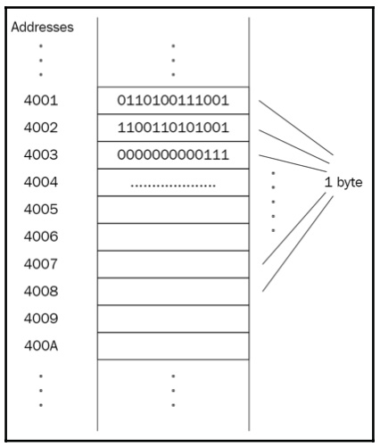
Memory consists of lots of boxes, each of which can store a specified amount of data. We will refer to these boxes as memory cells, considering that each cell can store 1 byte representing 8 bits. Each memory cell is unique, even if they store the same value. This uniqueness is achieved by addressing the cells so that each cell has its unique address in memory. The first cell has the address 0, the second cell 1, and so on.

The following diagram illustrates an excerpt of the memory, where each cell has a unique address and ability to store 1 byte of data:

Figure 1.9: Illustration of a memory cell

The preceding diagram can be used to abstractly represent both physical and virtual memories. The point of having an additional layer of abstraction is the ease of managing processes and providing more functionality than with physical memory. For example, OSs can execute programs greater than physical memory. Take a computer game as an example of a program that takes almost 2 GB of space and a computer with a physical memory of 512 MB. Virtual memory allows the OS to load the program portion by portion by unloading old parts from the physical memory and mapping new parts.

Virtual memory also better supports having more than one program in memory, thus supporting parallel (or pseudo-parallel) execution of multiple programs. This also provides efficient use of shared code and data, such as dynamic libraries. Whenever two different programs require the same library to work with, a single instance of the library could exist in memory and be used by both programs without them knowing about each other.

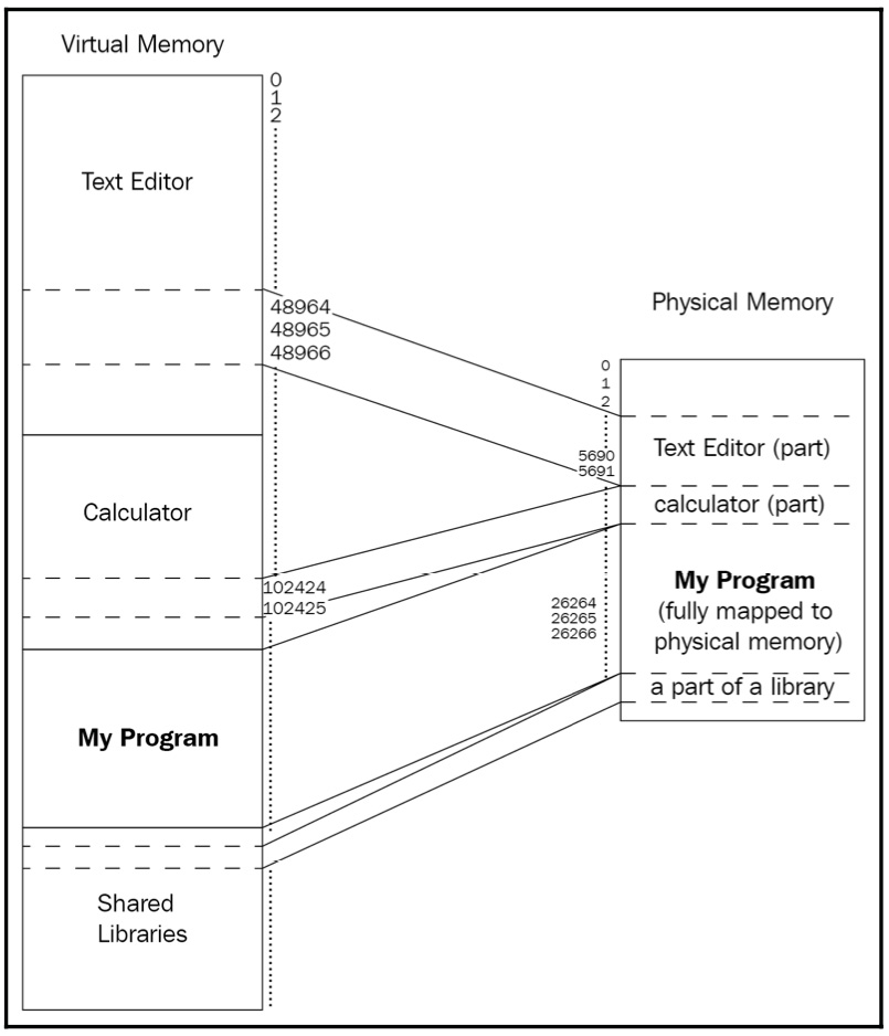
Let’s take a look at the following diagram, which depicts three programs loaded into memory:

Figure 1.10: Illustration of three different programs that have been loaded into memory

There are three running programs in the preceding diagram; each of the programs takes up some space in virtual memory. My Program is fully contained in the physical memory. while the Calculator and Text Editor are partially mapped to it.

Addressing

As mentioned earlier, each memory cell has a unique address, which guarantees the uniqueness of each cell. An address is usually represented in a hexadecimal form because it’s shorter and it’s faster to convert into binary rather than decimal numbers. A program that is loaded into virtual memory operates and sees logical addresses. These addresses, also called virtual addresses, are fake and provided by the OS, which translates them into physical addresses when needed. To optimize the translation, the CPU provides a translation lookaside buffer, a part of its memory management unit (MMU). The translation lookaside buffer caches recent translations of virtual addresses to physical addresses. So, efficient address translation is a software/hardware task. We will dive into the address’ structure and translation details in Chapter 5, Memory Management and Smart Pointers.

The length of the address defines the total size of memory that can be operated by the system. When you encounter statements such as a 32-bit system or a 64-bit system, this means the length of the address – that is, the address is 32 bits or 64 bits long. The longer the address, the bigger the memory. To make things clear, let’s compare an 8-bit long address with a 32-bit long one. As agreed earlier, each memory cell can store 1 byte of data and has a unique address. If the address length is 8 bits, the address of the first memory cell is all zeros – 0000 0000. The address of the next cell is greater by one – that is, it’s 0000 0001 – and so on.

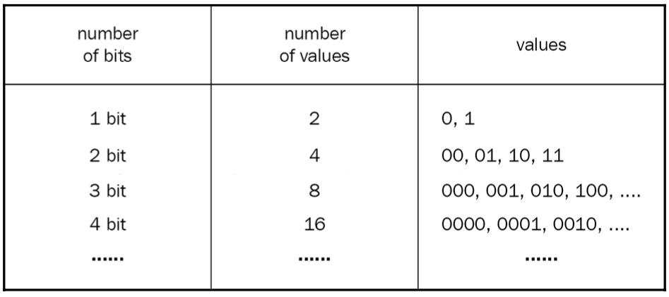
The biggest value that can be represented by 8 bits is 1111 1111. So, how many memory cells can be represented with an address length of 8 bits? This question is worth answering in more detail. How many different values can be represented by 1 bit? Two! Why? Because 1 bit can represent either 1 or 0. How many different values can be represented by 2 bits? Well, 00 is one value, 01 is another value, and then there’s 10, and, finally, 11. So, four different values in total can be represented by 2 bits.

Let’s make a table:

We can see a pattern here. Each position (each bit) in a number can have two values, so we can calculate the number of different values represented by N bits by finding 2N; therefore, the number of different values represented by 8 bits is 256. This means that an 8-bit system can address up to 256 memory cells. On the other hand, a 32-bit system can address 2^32 = 4 294 967 296 memory cells, each storing 1 byte of data – that is, storing 4294967296 * 1 byte = 4 GB of data.

Data types

What’s the point of having data types at all? Why can’t we program in C++ using some var keyword to declare variables and forget about variables such as short, long, int, char, wchar, and so on? Well, C++ does support a similar construct, known as the auto keyword, which we used previously in this chapter, a so-called placeholder type specifier. It’s named a placeholder because it is, indeed, a placeholder. We cannot (and we must not ever be able to) declare a variable and then change its type during runtime. The following code might be valid JavaScript code, but it is not valid C++ code:

var a = 12;
a = "Hello, World!";
a = 3.14;

Imagine the C++ compiler could compile this code. How many bytes of memory should be allocated for the a variable? When declaring var a = 12;, the compiler could deduce its type to int and specify 4 bytes of memory space, but when the variable changes its value to Hello, World!, the compiler has to reallocate the space or invent a new hidden variable named a1 of the std::string type. Then, the compiler tries to find every way to access the variable in the code that accesses it as a string and not as an integer or a double and replaces the variable with the hidden a1 variable. The compiler might just quit and start to ask itself the meaning of life.

We can declare something similar to the preceding code in C++ as follows:

auto a = 12;
auto b = "Hello, World!";
auto c = 3.14;

The difference between the previous two examples is that the second example declares three different variables of three different types. The previous non-C++ code declared just one variable and then assigned values of different types to it. You can’t change the type of a variable in C++, but the compiler allows you to use the auto placeholder and deduces the type of the variable by the value assigned to it.

It is crucial to understand that the type is deduced at compile time, while languages such as JavaScript allow you to deduce the type at runtime. The latter is possible because such programs are run in environments such as virtual machines, while the only environment that runs the C++ program is the OS. The C++ compiler must generate a valid executable file that could be copied into memory and run without a support system. This forces the compiler to know the actual size of the variable beforehand. Knowing the size is important to generate the final machine code because accessing a variable requires its address and size, and allocating memory space to a variable requires the number of bytes that it should take.

The C++ type system classifies types into two major categories:

• Fundamental types (int, double, char, void)
• Compound types (pointers, arrays, classes)

The language even supports special type traits, std::is_fundamental and std::is_compound, to find out the category of a type. Here is an example:

#include <iostream>
#include <type_traits>
struct Point {
    float x;
    float y; };
int main() {
std::cout << std::is_fundamental_v<Point> << " "
<< std::is_fundamental_v<int> << " "
<< std::is_compound_v<Point> << " "
<< std::is_compound_v<int> << std::endl;
}

Most of the fundamental types are arithmetic types such as int or double; even the char type is arithmetic. It holds a number rather than a character, as shown here:

char ch = 65;
std::cout << ch; // prints A

A char variable holds 1 byte of data, which means it can represent 256 different values (because 1 byte is 8 bits, and 8 bits can be used in 28 ways to represent a number). What if we use one of the bits as a sign bit, for example, allowing the type to support negative values as well? That leaves us with 7 bits for representing the actual value. Following the same logic, it allows us to represent 2^7 different values – that is, 128 (including 0) different values of positive numbers and the same amount of negative values. Excluding 0 gives us a range of -127 to +127 for the signed char variable. This signed versus unsigned representation applies to almost all integral types.

So, whenever you encounter that, for example, the size of an int is 4 bytes, which is 32 bits, you should already know that it is possible to represent the numbers 0 to 232 in an unsigned representation, and the values -231 to +231 in a signed representation.

Pointers

C++ is a unique language in the way that it provides access to low-level details such as addresses of variables. We can take the address of any variable declared in the program using the & operator, as shown here:

int answer = 42;
std::cout << &answer;

This code will output something similar to this:

0x7ffee1bd2adc

Notice the hexadecimal representation of the address. Although this value is just an integer, it is used to store it in a special variable called a pointer. A pointer is just a variable that can store address values and supports the * operator (dereferencing), allowing us to find the actual value stored at the address.

For example, to store the address of the variable answer in the preceding example, we can declare a pointer and assign the address to it:

int* ptr = &answer;

The variable answer is declared as int, which usually takes 4 bytes of memory space. We already agreed that each byte has a unique address. Can we conclude that the answer variable has four unique addresses? Well, yes and no. It does acquire four distinct but contiguous memory bytes, but when the address operator is used against the variable, it returns the address of its first byte. Let’s take a look at a portion of code that declares a couple of variables and then illustrate how they are placed in memory:

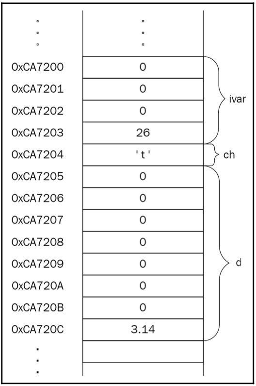
int ivar = 26;
char ch = 't';
double d = 3.14;

The size of a data type is implementation-defined, though the C++ standard states the minimum supported range of values for each type. Let’s suppose the implementation provides 4 bytes for int, 8 bytes for double, and 1 byte for char. The memory layout for the preceding code should look like this:

Figure 1.11: Variables in memory

Pay attention to ivar in the memory layout; it resides in four contiguous bytes.

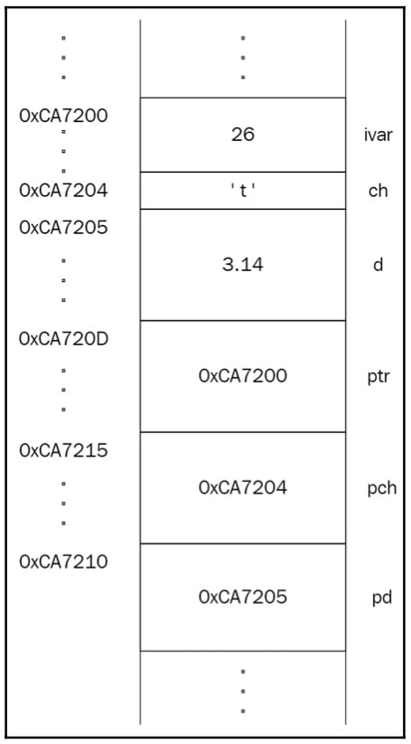
Whenever we take the address of a variable, whether it resides in a single byte or more than 1 byte, we get the address of the first byte of the variable. If the size doesn’t affect the logic behind the address operator, then why do we have to declare the type of the pointer? To store the address of ivar in the preceding example, we should declare the pointer as int*:

int* ptr = &ivar;
char* pch = &ch;
double* pd = &d;

The preceding code is depicted in the following diagram:

Figure 1.12: Illustration of a piece of memory that holds pointers that point to other variables

It turns out that the type of the pointer is crucial in accessing the variable using that very pointer. C++ provides the dereferencing operator for this (the * symbol before the pointer name):

std::cout << *ptr; // prints 26

It works like this:

1. It reads the contents of the pointer.
2. It finds the address of the memory cell that is equal to the address in the pointer.
3. It returns the value that is stored in that memory cell.

The question is, what if the pointer points to the data that resides in more than one memory cell? That’s where the pointer’s type comes in. When dereferencing the pointer, its type is used to determine how many bytes it should read and return, starting from the memory cell that it points to.

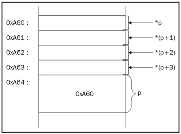
Now that we know that a pointer stores the address of the first byte of the variable, we can read any byte of the variable by moving the pointer forward. We should remember that the address is just a number, so adding or subtracting another number from it will produce another address. What if we point to an integer variable with a char pointer?

int ivar = 26;
char* p = (char*)&ivar;

When we try to dereference the p pointer, it will return only the first byte of ivar.

Now, if we want to move to the next byte of ivar, we can add 1 to the char pointer:

// the first byte
*p;
// the second byte
*(p + 1);
// the third byte
*(p + 2);
// dangerous stuff, the previous byte
*(p - 1);

Take a look at the following diagram; it clearly shows how we access bytes of the ivar integer:

Figure 1.13 Illustration of accessing the ivar integer’s bytes

If you want to read the first or the last two bytes, you can use a short pointer:

short* sh = (short*)&ivar;
// print the value in the first two bytes of ivar
std::cout << *sh;
// print the value in the last two bytes of ivar
std::cout << *(sh + 1);

Note

You should be careful with pointer arithmetics since adding or subtracting a number will move the pointer by the defined size of the data type. Adding 1 to an int pointer will add sizeof(int) * 1 to the actual address.

What about the size of a pointer? As mentioned previously, a pointer is just a variable that is special in the way that it can store a memory address and provide a dereferencing operator that returns the data located at that address. So, if the pointer is just a variable, it should reside in memory as well. We might consider that the size of a char pointer is less than the size of an int pointer just because the size of char is less than the size of int.

Here’s the catch: the data that is stored in the pointer has nothing to do with the type of data the pointer points to. Both the char and int pointers store the address of the variable, so to define the size of the pointer, we should consider the size of the address. The size of the address is defined by the system we work in. For example, in a 32-bit system, the address size is 32 bits long, and in a 64-bit system, the address size is 64 bits long. This leads us to a logical conclusion: the size of the pointer is the same regardless of the type of data it points to:

std::cout << sizeof(ptr) << " = "
<< sizeof(pch) << " = " << sizeof(pd);

It will output 4 = 4 = 4 in a 32-bit system and 8 = 8 = 8 in a 64-bit system.

Stack and the heap

The memory consists of segments and the program segments are distributed through these memory segments during loading. These are artificially divided ranges of memory addresses that make it easier to manage the program using the OS. A binary file is also divided into segments, such as code and data. We previously mentioned code and data as sections. Sections are the divisions of a binary file that are needed for the linker, which uses the sections that are meant for the linker to work and combines the sections that are meant for the loader into segments.

When we discuss a binary file from the runtime’s perspective, we mean segments. The data segment contains all the data required and used by the program, and the code segment contains the actual instructions that process the very same data. However, when we mention data, we don’t mean every single piece of data used in the program. Let’s take a look at this example:

#include <iostream>
int max(int a, int b) { return a > b ? a : b; }
int main() {
     std::cout << "The maximum of 11 and 22 is: " <<
       max(11, 22);
}

The code segment of the preceding program consists of the instructions of the main() and max() functions, where main() prints the message using the cout object’s operator<< and then calls the max() function. What data resides in the data segment? Does it contain the a and b arguments of the max() function? As it turns out, the only data that is contained in the data segment is the The maximum of 11 and 22 is: string, along with other static, global, or constant data. We didn’t declare any global or static variables, so the only data is the mentioned message.

The interesting thing comes with the 11 and 22 values. These are literal values, which means they have no address; therefore, they are not located anywhere in memory. If they are not located anywhere, the only logical explanation of how they are located within the program is that they reside in the code segment. They are a part of the max() call instruction.

What about the a and b arguments of the max() function? This is where the segment in virtual memory that is responsible for storing variables that have automatic storage duration comes in – the stack. As mentioned previously, the stack automatically handles allocating/deallocating memory space for local variables and function arguments. The a and b arguments will be located in the stack when the max() function is called. In general, if an object is said to have an automatic storage duration, the memory space will be allocated at the beginning of the enclosing block. So, when the function is called, its arguments are pushed into the stack:

int max(int a, int b) {
// allocate space for the "a" argument
 // allocate space for the "b" argument return a > b ? a :
 // b;
 // deallocate the space for the "a" argument // deallocate
 // the space for the "b" argument
}

When the function is done, the automatically allocated space will be freed at the end of the enclosing code block.

It’s said that the arguments (or local variables) are popped out of the stack. Push and pop are terms that are used within the context of the stack. You insert data into the stack by pushing it, and you retrieve (and remove) data out of the stack by popping it. You might have encountered the term last in, first out (LIFO). This perfectly describes the push and pop operations of the stack.

When the program is run, the OS provides the fixed size of the stack. The stack can grow in size and if it grows to the extent that no more space is left, it crashes because of the stack overflow.

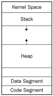
We described the stack as a manager of variables with automatic storage duration. The word automatic suggests that programmers shouldn’t care about the actual memory allocation and deallocation. Automatic storage duration can only be achieved if the size of the data or a collection of the data is known beforehand. This way, the compiler is aware of the number and type of function arguments and local variables. At this point, it seems more than fine, but programs tend to work with dynamic data – data of unknown size. We will study dynamic memory management in detail in Chapter 5, Memory Management and Smart Pointers; for now, let’s look at a simplified diagram of memory segments and find out what the heap is used for:

Figure 1.14: Simplified diagram of memory segments

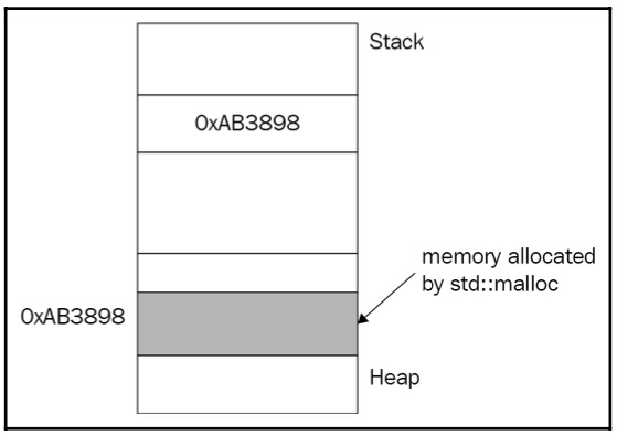
The program uses the heap segment to request more memory space than has been required before. This is done at runtime, which means the memory is allocated dynamically during the program execution. The program requests the OS for new memory space whenever required. The OS doesn’t know whether the memory is required for an integer, for a user-defined Point, or even for an array of user-defined Point. The program requests the memory by passing the actual size of bytes that it requires. For example, to request a space for an object of the Point type, the malloc() function can be used, as follows:

#include <cstdlib>
struct Point {
     float x;
     float y;
};
int main() {
     std::malloc(sizeof(Point));
}

The malloc() function allocates a contiguous memory space of sizeof(Point) bytes – let’s say 8 bytes. It then returns the address of the first byte of that memory as it is the only way to provide access to space. And the thing is, malloc() doesn’t know whether we requested memory space for a Point object or int, and it simply returns void*. void* stores the address of the first byte of allocated memory, but it definitely cannot be used to fetch the actual data by dereferencing the pointer, simply because void does not define the size of the data. Take a look at the following diagram; it shows that malloc allocates memory on the heap:

Figure 1.15: Memory allocation on the heap

To use the memory space, we need to cast the void pointer to the desired type:

Point* p = static_cast<Point*>(std::malloc(sizeof(Point)));

C++ solves this headache with the new operator, which automatically fetches the size of the memory space to be allocated and converts the result into the desired type:

Point* p = new Point;

Control flow

It’s hard to imagine a program that doesn’t contain a conditional statement. It’s almost a habit to check the input arguments of functions to secure their safe execution. For example, the divide() function takes two arguments, divides one by the other, and returns the result. It’s pretty clear that we need to make sure that the divisor is not zero:

int divide(int a, int b) {
    if (b == 0) {
        throw std::invalid_argument("The divisor is zero");
    }
    return a / b;
}

Conditionals are at the core of programming languages; after all, a program is a collection of actions and decisions. For example, the code at https://github.com/PacktPublishing/Expert-C-2nd-edition/tree/main/Chapter%2001/6_max.cpp uses conditional statements to find the maximum value out of two input arguments.

The preceding example is oversimplified on purpose to express the usage of the if-else statement as-is. However, what interests us the most is the implementation of such a conditional statement. What does the compiler generate when it encounters an if statement? The CPU executes instructions sequentially one by one, and instructions are simple commands that do exactly one thing. We can use complex expressions in a single line in a high-level programming language such as C++, while the assembly instructions are simple commands that can do only one simple operation in one cycle: move, add, subtract, and so on.

The CPU fetches the instruction from the code memory segment, decodes it to find out what it should do (move data, add numbers, or subtract them), and executes the command.

To run at its fastest, the CPU stores the operands and the result of the execution in storage units called registers. You can think of registers as temporary variables of the CPU. Registers are physical memory units that are located within the CPU so that access is much faster compared to the RAM. To access the registers from an assembly language program, we use their specified names, such as rax, rbx, rdx, and so on. The CPU commands operate on registers rather than the RAM cells; that’s why the CPU has to copy the contents of the variable from the memory to registers, execute operations and store the results in a register, and then copy the value of the register back to the memory cell.

For example, the following C++ expression takes just a single line of code:

a = b + 2 * c - 1;

This would look similar to the following assembly representation (comments are added after semicolons):

mov rax, b; copy the contents of "b"
 ; located in the memory to the register rax
mov rbx, c
; the same for the "c" to be able to calculate 2 * c
mul rbx, 2
; multiply the value of the rbx register with
; immediate value 2 (2 * c)
add rax, rbx; add rax (b) with rbx (2*c) and store back in the rax sub rax, 1; subtract 1 from rax
mov a, rax
; copy the contents of rax to the "a" located in the memory

A conditional statement suggests that a portion of the code should be skipped. For example, calling max(11, 22) means the if block will be omitted. To express this in the assembly language, the idea of jumps is used. We compare two values and, based on the result, we jump to a specified portion of the code. We label the portion to make it possible to find the set of instructions. For example, to skip adding 42 to the rbx register, we can jump to the portion labeled UNANSWERED using the unconditional jump instruction, jpm, as shown here:

mov rax, 2
 mov rbx, 0
 jmp UNANSWERED
 add rbx, 42; will be skipped UNANSWERED:
     add rax, 1
     ; ...

The jmp instruction performs an unconditional jump; this means it starts executing the first instruction at a specified label without any condition check. The good news is that the CPU provides conditional jumps as well. The body of the max() function will translate into the following assembly code (simplified), where the jg and jle commands are interpreted as jump if greater than and jump if less than or equal, respectively (based on the results of the comparison using the cmp instruction):

mov rax, max; copy the "max" into the rax register
 mov rbx, a
 mov rdx, b
 cmp rbx, rdx; compare the values of rbx and rdx (a and b)
jg GREATER; jump if rbx is greater than rdx (a > b)
jl LESSOREQUAL; jump if rbx is lesser than GREATER:
mov rax, rbx; max = a LESSOREQUAL:
mov rax, rdx; max = b

In the preceding code, the GREATER and LESSOREQUAL labels represent the if and else clauses of the max() function we implemented earlier.

Replacing conditionals with function pointers

Previously, we looked at memory segments, and one of the most important segments is the code segment (also called a text segment). This segment contains the program image, which is the instructions for the program that should be executed. Instructions are usually grouped into functions, which provide us with a unique name that allows us to call them from other functions. Functions reside in the code segment of the executable file.

A function has its own address. We can declare a pointer that takes the address of the function and then use it later to call that function:

int get_answer() { return 42; }
int (*fp)() = &get_answer;
// int (*fp)() = get_answer; same as &get_answer

The function pointer can be called the same way as the original function:

get_answer(); // returns 42
fp(); // returns 42

Let’s suppose we are writing a program that takes two numbers and a character from the input and executes an arithmetic operation on the numbers. The operation is specified by the character, whether it’s +, -, *, or /. We implement four functions, add(), subtract(), multiply(), and divide(), and call one of them based on the value of the character’s input.

Instead of checking the value of the character in a bunch of if statements or a switch statement, we will map the type of the operation to the specified function using a hash table (you can find the code at https://github.com/PacktPublishing/Expert-C-2nd-edition/tree/main/Chapter%2001/7_calculating_with_hash_table.cpp).

As you can see, std::unordered_map maps char to a function pointer defined as (*)(int, int). That is, it can point to any function that takes two integers and returns an integer.

Details of OOP

C++ supports OOP, a paradigm that is built upon dissecting entities into objects that exist in a web of close intercommunication. Imagine a simple scenario in the real world where you pick a remote to change the TV channel. At least three different objects take part in this action: the remote, the TV, and, most importantly, you. To express these real-world objects and their relationship using a programming language, we aren’t forced to use classes, class inheritance, abstract classes, interfaces, virtual functions, and so on. These features and concepts make the process of designing and coding a lot easier as they allow us to express and share ideas elegantly, but they are not mandatory. As the creator of C++, Bjarne Stroustrup, says, “Not every program should be object-oriented.” To understand the high-level concepts and features of the OOP paradigm, we will try to look behind the scenes. Throughout this book, we will dive into the design of object-oriented programs. Understanding the essence of objects and their relationship, and then using them to design object-oriented programs, is one of the goals of this book.

Most of the time, we operate with a collection of data grouped under a certain name, thus making an abstraction. Variables such as is_military, speed, and seats don’t make much sense if they’re perceived separately. Grouping them under the name Spaceship changes the way we perceive the data stored in the variables. We now refer to the many variables packed as a single object. To do so, we use abstraction; that is, we collect the individual properties of a real-world object from the perspective of the observer. An abstraction is a key tool in the programmer’s toolchain as it allows them to deal with complexity. The C language introduced struct as a way to aggregate data, as shown in the following code:

struct Spaceship {
bool is_military;
int speed;
int seats;
};

Grouping data is somewhat necessary for OOP. Each group of data is referred to as an object.

C++ does its best to support compatibility with the C language. While C structs are just tools that allow us to aggregate data, C++ makes them equal to classes, allowing them to have constructors, virtual functions, inherit other structs, and so on. The only difference between struct and class is the default visibility modifier: public for structs and private for classes. There is usually no difference in using structs over classes or vice versa. OOP requires more than just data aggregation. To fully understand OOP, let’s find out how we would incorporate the OOP paradigm if we have only simple structs providing data aggregation and nothing more.

The central entity of an e-commerce marketplace such as Amazon or Alibaba is Product, which we represent in the following way:

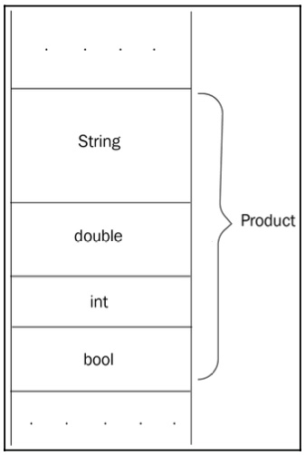
struct Product {
     std::string name;
     double price;
     int rating;
     bool available;
};

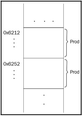
We will add more members to Product if necessary. The memory layout of an object of the Product type can be depicted like this:

Figure 1.16: The memory layout of a Product object

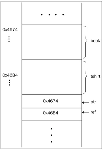
Declaring a Product object takes sizeof(Product) space in memory while declaring a pointer or a reference to the object takes the space required to store the address (usually 4 or 8 bytes). See the following code block:

Product book;
Product tshirt;
Product* ptr = &book;
Product& ref = tshirt;

We can depict the preceding code as follows:

Figure 1.17: Illustration of the Product pointer and the Product reference in memory

Let’s start with the space the Product object takes in memory. We can calculate the size of the Product object by summing the sizes of its member variables. The size of a boolean variable is 1 byte. The exact size of double or int is not specified in the C++ standard. In 64-bit machines, a double variable usually takes 8 bytes and an int variable takes 4 bytes.

The implementation of std::string is not specified in the standard, so its size depends on the library implementation. string stores a pointer to a character array, but it might also store the number of allocated characters to efficiently return it when size() is called. Some implementations of std::string take 8, 24, or 32 bytes of memory, but we will stick to 24 bytes in our example. By summing it up, the size of Product will be as follows:

24 (std::string) + 8 (double) + 4 (int) + 1 (bool) = 37 bytes.

Printing the size of Product outputs a different value:

std::cout << sizeof(Product);

It outputs 40 instead of the calculated 37 bytes. The reason behind the redundant bytes is the padding of the struct, a technique practiced by the compiler to optimize access to individual members of the object. The central processing unit (CPU) reads the memory in fixed-size words. The size of the word is defined by the CPU (usually, it’s 32 or 64 bits long). The CPU can access the data at once if it’s starting from a word-aligned address. For example, the boolean data member of Product requires 1 byte of memory and can be placed right after the rating member. As it turns out, the compiler aligns the data for faster access. Let’s suppose the word size is 4 bytes. This means that the CPU will access a variable without redundant steps if the variable starts from an address that’s divisible by 4. The compiler augments the struct earlier with additional bytes to align the members to word-boundary addresses.

High-level details of objects

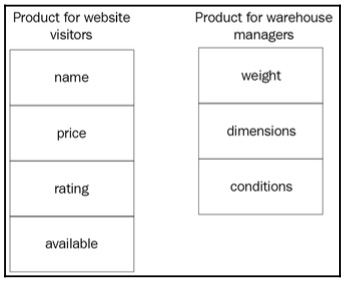
We deal with objects as entities representing the result of abstraction. We have already mentioned the role of the observer – that is, the programmer who defines the object based on the problem domain. The way the programmer defines this represents the process of abstraction. Let’s take an example of an eCommerce marketplace and its products. Two different teams of programmers might have different views of the same product. The team that implements the website cares about the properties of the object that are essential to website visitors: buyers. The properties that we showed earlier in the Product struct are mostly meant for website visitors, such as the selling price, the rating of the product, and so on. Programmers that implement the website touch the problem domain and verify the properties that are essential to defining a Product object.

The team that implements the online tools that help manage the products in the warehouse cares about the properties of the object that are essential in terms of product placement, quality control, and shipment. This team shouldn’t care about the rating of the product or even its price. This team mostly cares about the weight, dimensions, and conditions of the product. The following illustration shows the properties of interest:

Figure 1.18: The properties of interest for website visitors and warehouse managers

The first thing that programmers should do when starting the project is to analyze the problem and gather the requirements. In other words, they should get familiar with the problem domain and define the project requirements. The process of analyzing leads to defining objects and their types, such as the Product we discussed earlier. To get proper results from analyzing, we should think in objects, and, by thinking in objects, we mean considering the three main properties of objects: state, behavior, and identity.

Each object has a state that may or may not differ from the state of other objects. We’ve already introduced the Product struct, which represents an abstraction of a physical (or digital) product. All the members of a Product object collectively represent the state of the object. For example, Product contains members such as available, which is a Boolean; it equals true if the product is in stock. The values of the member variables define the state of the object. If you assign new values to the object member, its state will change:

Product cpp_book; // declaring the object
...
 // changing the state of the object cpp_book
cpp_book.available = true;
cpp_book.rating = 5;

The state of the object is the combination of all of its properties and values.

Identity is what differentiates one object from another. Even if we try to declare two physically indistinguishable objects, they will still have different names for their variables – that is, different identities:

Product book1;
book1.rating = 4;
book1.name = "Book";
Product book2;
book2.rating = 4;
book2.name = "Book";

The objects in the preceding example have the same state, but they differ by the names we refer to them by – that is, book1 and book2. Let’s say we could somehow create objects with the same name, as shown in the following code:

Product prod;
Product prod; // won't compile, but still "what if?"

If this was the case, they would still have different addresses in memory:

Figure 1.19: Illustration of a piece of memory that would hold variables with the same name if it was possible

In the previous examples, we assigned 5 and then 4 to the rating member variable. We can easily make things unexpectedly wrong by assigning invalid values to the object, like so:

cpp_book.rating = -12;

-12 is invalid in terms of the rating of a product and will confuse users if it’s allowed to. We can control the behavior of the changes made to the object by providing setter functions:

void set_rating(Product* p, int r) {
     if (r >= 1 && r <= 5) {
       p->rating = r;
     }
     // otherwise ignore
   }
...
 set_rating(&cpp_book, -12); // won't change the state

An object acts and reacts to requests from other objects. The requests are performed via function calls, which otherwise are called messages: an object passes a message to another. In the preceding example, the object that passed the corresponding set_rating message to the cpp_book object represents the object that we call the set_rating() function in. In this case, we suppose that we call the function from main(), which doesn’t represent any object at all. We could say it’s the global object, the one that operates the main() function, though there is not an entity like that in C++.

We distinguish the objects conceptually rather than physically. That’s the main point of thinking in terms of objects. The physical implementation of some concepts of OOP is not standardized, so we can name the Product struct as a class and claim that cpp_book is an instance of Product and that it has a member function called set_rating(). The C++ implementation almost does the same: it provides syntactically convenient structures (classes, visibility modifiers, inheritance, and so on) and translates them into simple structs with global functions such as set_rating() in the preceding example. Now, let’s dive into the details of the C++ object model.

Working with classes

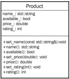
Classes make things a lot easier when dealing with objects. They do the simplest necessary thing in OOP: they combine data with functions for manipulating data. Let’s rewrite the example of the Product struct using a class and its powerful features (you can find the code at https://github.com/PacktPublishing/Expert-C-2nd-edition/tree/main/Chapter%2001/8_product.h).

The class declaration seems more organized, even though it exposes more functions than we use to define a similar struct. Here’s how we should illustrate the class:

Figure 1.20: UML diagram of a Product class

The preceding figure is somewhat special. As you can see, it has organized sections, signs before the names of functions, and so on. This type of diagram is called a unified modeling language (UML) class diagram. UML is a way to standardize the process of illustrating classes and their relationship. The first section is the name of the class (in bold), next comes the section for member variables, and then the section for member functions. The + (plus) sign in front of a function’s name means that the function is public. Member variables are usually private, but, if you need to emphasize this, you can use the - (minus) sign.

Initialization, destruction, copying, and moving

As shown previously, creating an object is a two-step process: memory allocation and initialization. Memory allocation is a result of an object declaration. C++ doesn’t care about the initialization of variables; it allocates the memory (whether it is automatic or manual) and it’s done. The actual initialization should be done by the programmer, which is why we have a constructor in the first place.

The same logic follows for the destructor. If we skip the declarations of the default constructor or destructor, the compiler should generate them implicitly; it will also remove them if they are empty (to eliminate redundant calls to empty functions). The default constructor will not be generated by the compiler if any constructor with parameters is declared, including the copy constructor. We can force the compiler to implicitly generate the default constructor:

class Product {
public:
     Product() = default;
// ...
};

We also can force it not to generate the compiler by using the delete specifier, as shown here:

class Product {
public:
     Product() = delete;
// ...
};

This will prohibit default-initialized object declarations – that is, Product p; won’t compile.

Object initialization happens when the object is created. Destruction usually happens when the object is no longer accessible. The latter may be tricky when the object is allocated on the heap. Take a look at the following code; it declares four Product objects in different scopes and segments of memory:

static Product global_prod; // #1
Product* foo() {
 Product* heap_prod = new Product(); // #4 heap_prod->name
                                     // = "Sample";
 return heap_prod;
}
int main() {
 Product stack_prod; // #2 if (true) {
Product tmp; // #3
       tmp.rating = 3;
     }
     stack_prod.price = 4.2;
foo();
}

global_prod has a static storage duration and is placed in the global/static section of the program; it is initialized before main() is called. When main() starts, stack_prod is allocated on the stack and will be destroyed when main() ends (the closing curly brace of the function is considered as its end). Though the conditional expression looks weird and too artificial, it’s a good way to express the block scope.

The tmp object will also be allocated on the stack, but its storage duration is limited to the scope it has been declared in: it will be automatically destroyed when the execution leaves the if block. That’s why variables on the stack have automatic storage duration. Finally, when the foo() function is called, it declares the heap_prod pointer, which points to the address of the Product object allocated on the heap.

The preceding code contains a memory leak because the heap_prod pointer (which itself has an automatic storage duration) will be destroyed when the execution reaches the end of foo(), while the object allocated on the heap won’t be affected. Don’t mix the pointer and the actual object it points to: the pointer just contains the address of the object, but it doesn’t represent the object.

When the function ends, the memory for its arguments and local variables, which is allocated on the stack, will be freed, but global_prod will be destroyed when the program ends – that is, after the main() function finishes. The destructor will be called when the object is about to be destroyed.

There are two kinds of copying: deep copying and shallow copying objects. The language allows us to manage copy-initialization and assigning objects with the copy constructor and the assignment operator. This is a necessary feature for programmers because we can control the semantics of copying. Take a look at the following example:

Product p1;
Product p2;
p2.set_price(4.2);
p1 = p2; // p1 now has the same price Product p3 = p2;
// p3 has the same price

The p1 = p2; line is a call to the assignment operator, while the last line is a call to the copy constructor. The equals sign shouldn’t confuse you regarding whether it’s an assignment or a copy constructor call. Each time you see a declaration followed by an assignment, consider it a copy construction. The same applies to the new initializer syntax (Product p3{p2};).

The compiler will generate the following code:

Product p1;
 Product p2;
Product_set_price(p2, 4.2);
operator=(p1, p2);
 Product p3;
Product_copy_constructor(p3, p2);

Temporary objects are everywhere in code. Most of the time, they are required to make the code work as expected. For example, when we add two objects together, a temporary object is created to hold the return value of operator+:

Warehouse small;
 Warehouse mid;
 // ... some data inserted into the small and mid objects
Warehouse large{small + mid}; // operator+(small, mid)

Let’s take a look at the implementation of the operator+() global for Warehouse objects:

// considering declared as friend in the Warehouse class Warehouse operator+(const Warehouse& a, const Warehouse& b) {
     Warehouse sum; // temporary
     sum.size_ = a.size_ + b.size_;
     sum.capacity_ = a.capacity_ + b.capacity_;
     sum.products_ = new Product[sum.capacity_];
     for (int ix = 0; ix < a.size_; ++ix) {
       sum.products_[ix] = a.products_[ix];
     }
     for (int ix = 0; ix < b.size_; ++ix) {
       sum.products_[a.size_ + ix] = b.products_[ix];
     }
     return sum;
}

The preceding implementation declares a temporary object and returns it after filling it with necessary data. The call in the previous example could be translated into the following:

Warehouse small;
 Warehouse mid;
 // ... some data inserted into the small and mid objects
Warehouse tmp{operator+(small, mid)};
 Warehouse large;
 Warehouse_copy_constructor(large, tmp);
__destroy_temporary(tmp);

Move semantics, which was introduced in C++11, allow us to skip the temporary creation by moving the return value into the Warehouse object. To do so, we should declare a move constructor for Warehouse, which can distinguish between temporaries and treat them efficiently:

class Warehouse {
public:
Warehouse(); // default constructor
Warehouse(const Warehouse&); // copy constructor Warehouse(Warehouse&&); // move constructor
 // code omitted for brevity
};

Class relationships

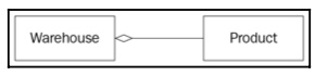
Object intercommunication is at the heart of object-oriented systems. The relationship is the logical link between objects. The way we can distinguish or set up a proper relationship between classes of objects defines both the performance and quality of the system design overall. Consider the Product and Warehouse classes; they are in a relationship called aggregation because Warehouse contains products – that is, Warehouse aggregates Product:

Figure 1.21: A UML diagram that depicts aggregation between Warehouse and Product

There are several kinds of relationships in terms of pure OOP, such as association, aggregation, composition, instantiation, generalization, and others.

Aggregation and composition

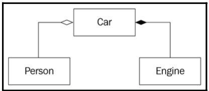
We encountered aggregation in the example of the Warehouse class. The Warehouse class stores an array of products. In more general terms, it can be called an association, but to strongly emphasize the exact containment, we use the term aggregation or composition. In the case of aggregation, the class that contains an instance or instances of other classes could be instantiated without the aggregate. This means that we can create and use a Warehouse object without necessarily creating Product objects contained in Warehouse. Another example of aggregation is Car and Person. A Car object can contain a Person object (as a driver or passenger) since they are associated with each other, but the containment is not strong. We can create a Car object without a Driver object in it (you can find the code at https://github.com/PacktPublishing/Expert-C-2nd-edition/tree/main/Chapter%2001/9_car_person_aggregation.h).

Strong containment is expressed by composition. For the Car example, an object of the Engine class is required to make a complete Car object. In this physical representation, the Engine member is automatically created when a Car object is created.

The following is the UML representation of aggregation and composition:

Figure 1.22: A UML diagram that demonstrates examples of aggregation and composition

When designing classes, we have to decide on their relationship. The best way to define the composition between the two classes is the has-a relationship test. A Car object has-a Engine member because a car has an engine. Any time you can’t decide whether the relationship should be expressed in terms of composition, ask the has-a question. Aggregation and composition are somewhat similar; they just describe the strength of the connection. For aggregation, the proper question would be can have a; for example, a Car object can have a Driver object (of the Person type); that is, the containment is weak.

Inheritance

Inheritance is a programming concept that allows us to reuse classes. Programming languages provide different implementations of inheritance, but the general rule always stands: the class relationship should answer the is-a question. For example, a Car object is-a Vehicle class, which allows us to inherit Car from Vehicle:

class Vehicle {
   public:
     void move();
   };
class Car : public Vehicle { public: Car();
// ...
};

Car now has the move() member function derived from Vehicle. Inheritance itself represents a generalization/specialization relationship, where the parent class (Vehicle) is the generalization and the child class (Car) is the specialization.

You should only consider using inheritance if it is necessary. As we mentioned earlier, classes should satisfy the is-a relationship, and sometimes, this is a bit tricky.