-
Book Overview & Buying
-
Table Of Contents

Learn Quantum Computing with Python and IBM Quantum Experience
By :
Learn Quantum Computing with Python and IBM Quantum Experience
By:
Overview of this book
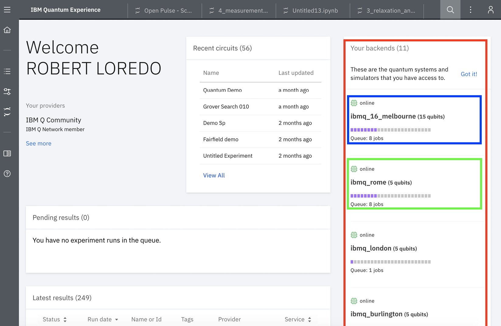
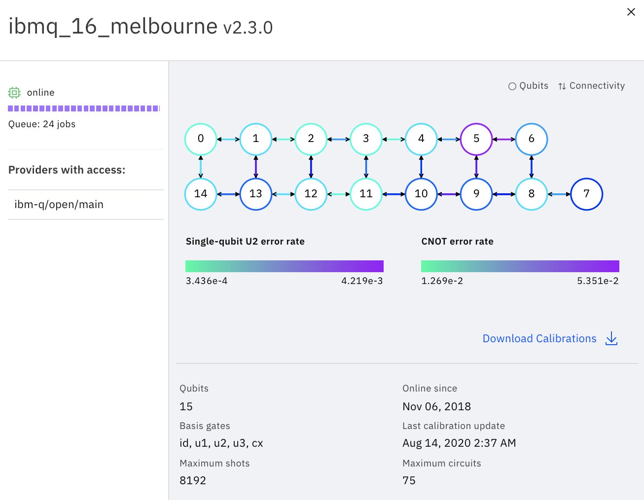
IBM Quantum Experience is a platform that enables developers to learn the basics of quantum computing by allowing them to run experiments on a quantum computing simulator and a real quantum computer. This book will explain the basic principles of quantum mechanics, the principles involved in quantum computing, and the implementation of quantum algorithms and experiments on IBM's quantum processors.
You will start working with simple programs that illustrate quantum computing principles and slowly work your way up to more complex programs and algorithms that leverage quantum computing. As you build on your knowledge, you’ll understand the functionality of IBM Quantum Experience and the various resources it offers. Furthermore, you’ll not only learn the differences between the various quantum computers but also the various simulators available. Later, you’ll explore the basics of quantum computing, quantum volume, and a few basic algorithms, all while optimally using the resources available on IBM Quantum Experience.
By the end of this book, you'll learn how to build quantum programs on your own and have gained practical quantum computing skills that you can apply to your business.
Table of Contents (21 chapters)
Preface

Section 1: Tour of the IBM Quantum Experience (QX)
 Free Chapter
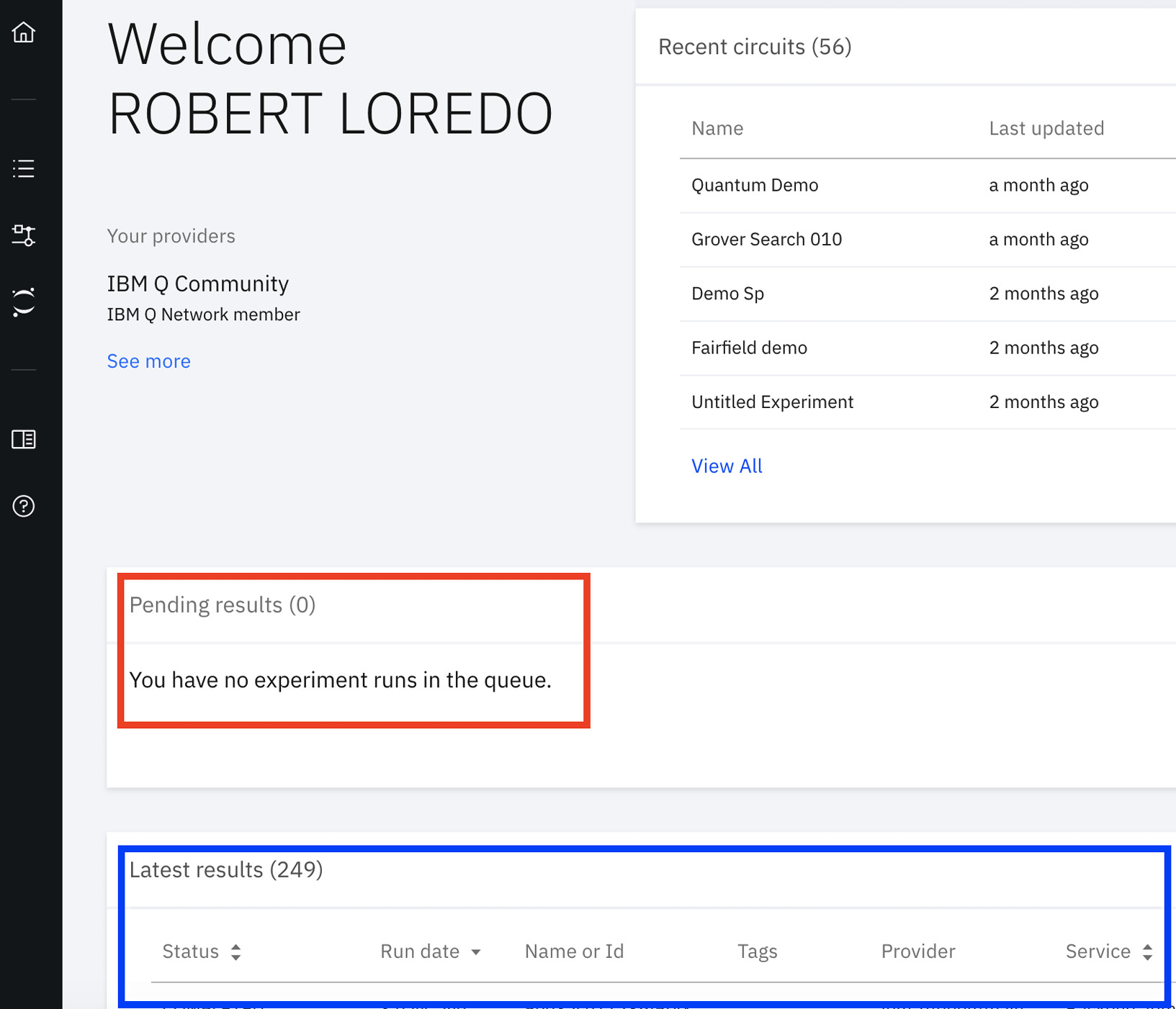
Chapter 1: Exploring the IBM Quantum Experience
Chapter 2: Circuit Composer – Creating a Quantum Circuit
Chapter 3: Creating Quantum Circuits using Quantum Lab Notebooks
Section 2: Basics of Quantum Computing
Chapter 4: Understanding Basic Quantum Computing Principles
Chapter 5: Understanding the Quantum Bit (Qubit)
Chapter 6: Understanding Quantum Logic Gates
Section 3: Algorithms, Noise, and Other Strange Things in Quantum World
Chapter 7: Introducing Qiskit and its Elements
Chapter 8: Programming with Qiskit Terra
Chapter 9: Monitoring and Optimizing Quantum Circuits
Chapter 10: Executing Circuits Using Qiskit Aer
Chapter 11: Mitigating Quantum Errors Using Ignis
Chapter 12: Learning about Qiskit Aqua
Chapter 13: Understanding Quantum Algorithms
Chapter 14: Applying Quantum Algorithms
Assessments
Other Books You May Enjoy
Appendix A: Resources