Supervised Machine Learning with Python

For this chapter, you will need to install the following software, if you haven't already done so:

The code files for this chapter can be found athttps:/​/​github.​com/​PacktPublishing/Supervised-Machine-Learning-with-Python.

First, we will take a look at what we can do with supervised machine learning. With the following Terminal prompt, we will launch a new Jupyter Notebook:

jupyter notebook

Once we are inside this top-level, Hands-on-Supervised-Machine-Learning-with-Python-master home directory, we will go directly inside the examples directory:

You can see that our only Notebook in here is 1.1 Supervised Learning Demo.ipynb:

We have the supervised learning demo Jupyter Notebook. We are going to be using a UCI dataset called the Spam dataset. This is a list of different emails that contain different features that correspond to spam or not spam. We want to build a machine learning algorithm that can predict whether or not we have an email coming in that is going to be spam. This could be extremely helpful for you if you're running your own email server.

So, the first function in the following code is simply a request's get function. You should already have the dataset, which is already sitting inside the examples directory. But in case you don't, you can go ahead and run the following code. You can see that we already have spam.csv, so we're not going to download it:

from urllib.request import urlretrieve, ProxyHandler, build_opener, install_opener
import requests
import os
pfx = "https://archive.ics.uci.edu/ml/machine-learning databases/spambase/"
data_dir = "data"
# We might need to set a proxy handler...
try:
    proxies = {"http": os.environ['http_proxy'],
               "https": os.environ['https_proxy']}
    print("Found proxy settings")
    #create the proxy object, assign it to a variable
    proxy = ProxyHandler(proxies)
    # construct a new opener using your proxy settings
    opener = build_opener(proxy)
    # install the opener on the module-level
    install_opener(opener)

except KeyError:
    pass
# The following will download the data if you don't already have it...
def get_data(link, where):
    # Append the prefix
    link = pfx + link

Next, we will use the pandas library. This is a data analysis library from Python. You can install it when we go through the next stage, which is the environment setup. This library is a data frame data structure that is a kind of native Python, which we will use as follows:

import pandas as pd
names = ["word_freq_make", "word_freq_address", "word_freq_all", 
         "word_freq_3d", "word_freq_our", "word_freq_over", 
         "word_freq_remove", "word_freq_internet", "word_freq_order",
         "word_freq_mail", "word_freq_receive", "word_freq_will", 
         "word_freq_people", "word_freq_report", "word_freq_addresses", 
         "word_freq_free", "word_freq_business", "word_freq_email", 
         "word_freq_you", "word_freq_credit", "word_freq_your", 
         "word_freq_font", "word_freq_000", "word_freq_money", 
         "word_freq_hp", "word_freq_hpl", "word_freq_george", 
         "word_freq_650", "word_freq_lab", "word_freq_labs", 
         "word_freq_telnet", "word_freq_857", "word_freq_data", 
         "word_freq_415", "word_freq_85", "word_freq_technology", 
         "word_freq_1999", "word_freq_parts", "word_freq_pm", 
         "word_freq_direct", "word_freq_cs", "word_freq_meeting", 
         "word_freq_original", "word_freq_project", "word_freq_re", 
         "word_freq_edu", "word_freq_table", "word_freq_conference", 
         "char_freq_;", "char_freq_(", "char_freq_[", "char_freq_!", 
         "char_freq_$", "char_freq_#", "capital_run_length_average", 
         "capital_run_length_longest", "capital_run_length_total",
         "is_spam"]
df = pd.read_csv(os.path.join("data", "spam.csv"), header=None, names=names)
# pop off the target
y = df.pop("is_spam")
df.head()

This allows us to lay out our data in the following format. We can use all sorts of different statistical functions that are nice to use when you're doing machine learning:

If some of this terminology is not familiar to you, don't panic yet—we will learn about these terminologies in detail over the course of the book.

For train_test_split, we will take the df dataset and split it into two parts: train set and test set. In addition to that, we have the target, which is a 01 variable that indicates true or false for spam or not spam. We will split that as well, which includes the corresponding vector of true or false labels. By splitting the labels, we get 3680 training samples and 921 test samples, file as shown in the following code snippet:

from sklearn.model_selection import train_test_split
X_train, X_test, y_train, y_test = train_test_split(df, y, test_size=0.2, random_state=42, stratify=y)
print("Num training samples: %i" % X_train.shape[0])
print("Num test samples: %i" % X_test.shape[0])

The output of the preceding code is as follows:

Num training samples: 3680
Num test samples: 921

In the following code, we have the packtml library. This is the actual package that we are building, which is a classification and regression tree classifier. CARTClassifier is simply a generalization of a decision tree for both regression and classification purposes. Everything we fit here is going to be a supervised machine learning algorithm that we build from scratch. This is one of the classifiers that we are going to build in this book. We also have this utility function for plotting a learning curve. This is going to take our train set and break it into different folds for cross-validation. We will fit the training set in different stages of numbers of training samples, so we can see how the learning curve converges between the train and validation folds, which determines how our algorithm is learning, essentially:

from packtml.utils.plotting import plot_learning_curve
from packtml.decision_tree import CARTClassifier
from sklearn.metrics import accuracy_score
import numpy as np
import matplotlib.pyplot as plt
%matplotlib inline

# very basic decision tree
plot_learning_curve(
        CARTClassifier, metric=accuracy_score,
        X=X_train, y=y_train, n_folds=3, seed=21, trace=True,
        train_sizes=(np.linspace(.25, .75, 4) * X_train.shape[0]).astype(int),
        max_depth=8, random_state=42)\
    .show()

We will go ahead and run the preceding code and plot how the algorithm has learned across the different sizes of our training set. You can see we're going to fit it for 4 different training set sizes at 3 folds of cross-validation.

So, what we're actually doing is fitting 12 separate models, which will take a few seconds to run:

In the preceding output, we can see our Training score and our Validation score. The Training score diminishes as it learns to generalize, and our Validation score increases as it learns to generalize from the training set to the validation set. So, our accuracy is hovering right around 92-93% on our validation set.

We will use the hyperparameters from the very best one here:

decision_tree = CARTClassifier(X_train, y_train, random_state=42, max_depth=8)

Logistic regression

In this section, we will learn about logistic regression, which is another classification model that we're going to build from scratch. We will go ahead and fit the following code:

from packtml.regression import SimpleLogisticRegression
# simple logistic regression classifier
plot_learning_curve(
        SimpleLogisticRegression, metric=accuracy_score,
        X=X_train, y=y_train, n_folds=3, seed=21, trace=True,
        train_sizes=(np.linspace(.25, .8, 4) *     X_train.shape[0]).astype(int),
        n_steps=250, learning_rate=0.0025, loglik_interval=100)\
    .show()

This is much faster than the decision tree. In the following output, you can see that we converge a lot more around the 92.5% range. This looks a little more consistent than our decision tree, but it doesn't perform quite well enough on the validation set:

In the following screenshot, there are encoded records of spam emails. We will see how this encoding performs on an email that we can read and validate. So, if you have visited the UCI link that was included at the top of the Jupyter Notebook, it will provide a description of all the features inside the dataset. We have a lot of different features here that are counting the ratio of particular words to the number of words in the entire email. Some of those words might be free and some credited. We also have a couple of other features that are counting character frequencies, the number of exclamation points, and the number of concurrent capital runs.

So, if you have a really highly capitalized set of words, we have all these features:

In the following screenshot, we will create two emails. The first email is very obviously spam. Even if anyone gets this email, no one will respond to it:

spam_email = """
Dear small business owner,

This email is to inform you that for $0 down, you can receive a 
FREE CREDIT REPORT!!! Your money is important; PROTECT YOUR CREDIT and 
reply direct to us for assistance!
"""

print(spam_email)

The output of the preceding code snippet is as follows:

Dear small business owner,

This email is to inform you that for $0 down, you can receive a 
FREE CREDIT REPORT!!! Your money is important; PROTECT YOUR CREDIT and 
reply direct to us for assistance!

The second email looks less like spam:

The model that we have just fit is going to look at both of the emails and encode the features, and will classify which is, and which is not, spam.

The following function is going to encode those emails into the features we discussed. Initially, we're going to use a Counter function as an object, and tokenize our emails. All we're doing is splitting our email into a list of words, and then the words can be split into a list of characters. Later, we'll count the characters and words so that we can generate our features:

from collections import Counter
import numpy as np
def encode_email(email):
    # tokenize the email
    tokens = email.split()

    # easiest way to count characters will be to join everything
    # up and split them into chars, then use a counter to count them
    # all ONE time.
    chars = list("".join(tokens))
    char_counts = Counter(chars)
    n_chars = len(chars)

    # we can do the same thing with "tokens" to get counts of words
    # (but we want them to be lowercase!)
    word_counts = Counter([t.lower() for t in tokens])

    # Of the names above, the ones that start with "word" are
    # percentages of frequencies of words. Let's get the words
    # in question
    freq_words = [ 
        name.split("_")[-1]
        for name in names 
        if name.startswith("word")
    ]

    # compile the first 48 values using the words in question
    word_freq_encodings = [100. * (word_counts.get(t, 0) / len(tokens))
                           for t in freq_words]

 

So, all those features that we have up at the beginning tell us what words we're interested in counting. We can see that the original dataset is interested in counting words such as address, email, business, and credit, and then, for our characters, we're looking for opened and closed parentheses and dollar signs (which are quite relevant to our spam emails). So, we're going to count all of those shown as follows:

Apply the ratio and keep track of the total number of capital_runs, computing the mean average, maximum, and minimum:

 # make a np array to compute the next few stats quickly
capital_runs = np.asarray(capital_runs)
    capital_stats = [capital_runs.mean(), 
                     capital_runs.max(), 
                     capital_runs.sum()]

When we run the preceding code, we get the following output. This is going to encode our emails. This is just simply a vector of all the different features. It should be about 50 characters long:

# get the email vectors
fake_email = encode_email(spam_email)
real_email = encode_email(not_spam)
# this is what they look like:
print("Spam email:")
print(fake_email)
print("\nReal email:")
print(real_email)

The output of the preceding code is as follows:

When we fit the preceding values into our models, we will see whether our model is any good. So, ideally, we will see that the actual fake email is predicted to be fake, and the actual real email is predicted to be real. So, if the emails are predicted as fake, our spam prediction is indeed spam for both the decision tree and the logistic regression. Our true email is not spam, which perhaps is even more important, because we don't want to filter real email into the spam folder. So, you can see that we fitted some pretty good models here that apply to something that we would visually inspect as true spam or not:

predict = (lambda rec, mod: "SPAM!" if mod.predict([rec])[0] == 1 else "Not spam")

print("Decision tree predictions:")
print("Spam email prediction: %r" % predict(fake_email, decision_tree))
print("Real email prediction: %r" % predict(real_email, decision_tree))

print("\nLogistic regression predictions:")
print("Spam email prediction: %r" % predict(fake_email, logistic_regression))
print("Real email prediction: %r" % predict(real_email, logistic_regression))

The output of the preceding code is as follows:

This is a demo of the actual algorithms that we're going to build from scratch in this book, and can be applied to real-world problems.

We will go ahead and get our environment set up. Now that we have walked through the preceding example, let's go ahead and get our Anaconda environment set up. Among other things, Anaconda is a dependency management tool that will allow us to control specific versioning of each of the packages that we want to use. We will go to the Anaconda website through this link, https://www.anaconda.com/download/, and click on the Download tab.

Once you have Anaconda set up inside the home directory, we are going to use the environment.yml file. You can see that the name of the environment we're going to create is packt-sml for supervised machine learning. We will need NumPy, SciPy, scikit-learn, and pandas. These are all scientific computing and data analysis libraries. Matplotlib is what we were using to plot those plots inside the Jupyter Notebook, so you're going to need all those plots. The conda package makes it really easy to build this environment. All we have to do is type conda env create and then -f to point it to the file, go to Hands-on-Supervised-Machine-Learning-with-Python-master, and we're going to use the environment.yml as shown in the following command:

cat environment.yml
conda env create -f environment.yml

As this is the first time you're creating this, it will create a large script that will download everything you need. Once you have created your environment, you need to activate it. So, on a macOS or a Linux machine, we will type source activate packt-sml.

If you're on Windows, simply type activate packt-sml, which will activate that environment:

 source activate packt-sml

The output is as follows:

In order to build the package, we will type the cat setup.py command. We can inspect this quickly:

cat setup.py

Take a look at this setup.py. Basically, this is just using setup tools to install the package. In the following screenshot, we see all the different sub models:

We will build the package by typing the python setup.py install command. Now, when we go into Python and try to import packtml, we get the following output:

In this section, we have installed the environment and built the package. In the next section, we will start covering some of the theory behind supervised machine learning.

In this section, we will formally define what machine learning is and, specifically, what supervised machine learning is.

In the early days of AI, everything was a rules engine. The programmer wrote the function and the rules, and the computer simply followed them. Modern-day AI is more in line with machine learning, which teaches a computer to write its own functions. Some may contest that oversimplification of the concept, but, at its core, this is largely what machine learning is all about.

We're going to look at a quick example of what machine learning is and what it is not. Here, we're using scikit-learn's datasets, submodule to create two objects and variables, also known as covariance or features, which are along the column axis. y is a vector with the same number of values as there are rows in X. In this case, y is a class label. For the sake of an example, y here could be a binary label corresponding to a real-world occurrence, such as the malignancy of a tumor.X is then a matrix of attributes that describe y. One feature could be the diameter of the tumor, and another could indicate its density. The preceding explanation can be seen in the following code:

import numpy as np
from sklearn.datasets import make_classification

rs = np.random.RandomState(42)
X,y = make_classification(n_samples=10, random_state=rs)

A rules engine, by our definition, is simply business logic. It can be as simple or as complex as you need it to be, but the programmer makes the rules. In this function, we're going to evaluate our X matrix by returning 1, or true, where the sums over the rows are greater than 0. Even though there's some math involved here, there is still a rules engine, because we, the programmers, defined a rule. So, we could theoretically get into a gray area, where the rule itself was discovered via machine learning. But, for the sake of argument, let's take an example that the head surgeon arbitrarily picks 0 as our threshold, and anything above that is deemed as cancerous:

def make_life_alterning_decision(X):
    """Determine whether something big happens"""
    row_sums = X.sum(axis=1)
    return (row_sums > 0).astype(int)
make_life_alterning_decision(X)

The output of the preceding code snippet is as follows:

array([0, 1, 0, 0, 1, 1, 1, 0, 1, 0])

Now, as mentioned before, our rules engine can be as simple or as complex as we want it to be. Here, we're not only interested in row_sums, but we have several criteria to meet in order to deem something cancerous. The minimum value in the row must be less than -1.5, in addition to one or more of the following three criteria:

So, even though our math is a little more complex here, we're still just building a rules engine:

def make_more_complex_life_alterning_decision(X):
    """Make a more complicated decision about something big"""   
    row_sums = X.sum(axis=1)
      return ((X.min(axis=1) < -1.5) &
              ((row_sums >= 0.) |
               (row_sums % 0.5 == 0) |
               (X.max(axis=1) > 1.5))).astype(int)

make_more_complex_life_alterning_decision(X) 

The output of the preceding code is as follows:

array([0, 1, 1, 1, 1, 1, 0, 1, 1, 0])

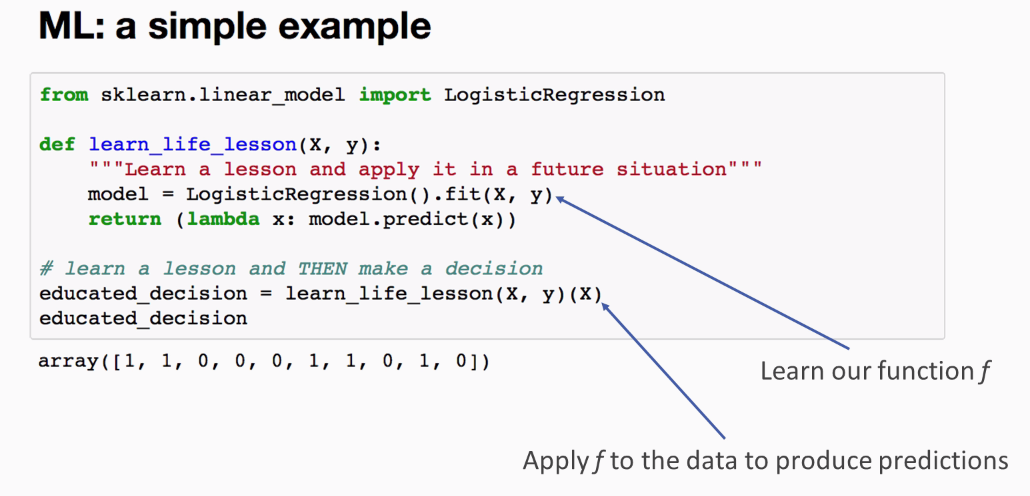
Now, let's say that our surgeon understands and realizes they're not the math or programming whiz that they thought they were. So, they hire programmers to build them a machine learning model. The model itself is a function that discovers parameters that complement a decision function, which is essentially the function the machine itself learned. So, parameters are things we'll discuss in our next Chapter 2, Implementing Parametric Models, which are parametric models. So, what's happening behind the scenes when we invoke the fit method is that the model learns the characteristics and patterns of the data, and how the X matrix describes the y vector. Then, when we call the predict function, it applies its learned decision function to the input data to make an educated guess:

from sklearn.linear_model import LogisticRegression

def learn_life_lession(X, y):
    """Learn a lesson abd apply it in a future situation"""
    model = LogisticRegression().fit(X, y)
    return (lambda X: model.predict(X))
educated_decision = learn_life_lession(X, y)(X)
educated_decision

The output of the preceding code is as follows:

array([1, 1, 0, 0, 0, 1, 1, 0, 1, 0])

So, now we're at a point where we need to define specifically what supervised learning is. Supervised learning is precisely the example we just described previously. Given our matrix of examples, X, in a vector of corresponding labels, y, that learns a function which approximates the value of y or

:

There are other forms of machine learning that are not supervised, known asunsupervised machine learning. These do not have labels and are more geared toward pattern recognition tasks. So, what makes something supervised is the presence of labeled data.

Going back to our previous example, when we invoke the fit method, we learn our new decision function and then, when we call predict, we're approximating the new y values. So, the output is this

 we just looked at:

Supervised learning learns a function from labelled samples that approximates future y values. At this point, you should feel comfortable explaining the abstract concept—just the high-level idea of what supervised machine learning is.

In the last section, we got comfortable with the idea of supervised machine learning. Now, we will learn how exactly a machine learns underneath the hood. This section is going to examine a common optimization technique used by many machine learning algorithms, called hill climbing. It is predicated on the fact that each problem has an ideal state and a way to measure how close or how far we are from that. It is important to note that not all machine learning algorithms use this approach.

Loss functions

First, we'll cover loss functions, and then, prior to diving into hill climbing and descent, we'll take a quick math refresher.

Note

There's going to be some math in this lesson, and while we try to shy away from the purely theoretical concepts, this is something that we simply have to get through in order to understand the guts of most of these algorithms. There will be a brief applied section at the end. Don't panic if you can't remember some of the calculus; just simply try to grasp what is happening behind the black box.

So, as mentioned before, a machine learning algorithm has to measure how close it is to some objective. We define this as a cost function, or a loss function. Sometimes, we hear it referred to as an objective function. Although not all machine learning algorithms are designed to directly minimize a loss function, we're going to learn the rule here rather than the exception. The point of a loss function is to determine the goodness of a model fit. It is typically evaluated over the course of a model's learning procedure and converges when the model has maximized its learning capacity.

A typical loss function computes a scalar value which is given by the true labels and the predicted labels. That is, given our actual y and our predicted y, which is

. This notation might be cryptic, but all it means is that some function, L, which we're going to call our loss function, is going to accept the ground truth, which is y and the predictions, 

, and return some scalar value. The typical formula for the loss function is given as follows:

So, I've listed several common loss functions here, which may or may not look familiar. Sum of Squared Error (SSE) is a metric that we're going to be using for our regression models:

Cross entropy is a very commonly used classification metric:

In the following diagram, the L function on the left is simply indicating that it is our loss function over y and

 given parameter theta. So, for any algorithm, we want to find the set of the theta parameters that minimize the loss. That is, if we're predicting the cost of a house, for example, we may want to estimate the cost per square foot as accurately as possible so as to minimize how wrong we are.

Parameters are often in a much higher dimensional space than can be represented visually. So, the big question we're concerned with is the following: How can we minimize the cost? It is typically not feasible for us to attempt every possible value to determine the true minimum of a problem. So, we have to find a way to descend this nebulous hill of loss. The tough part is that, at any given point, we don't know whether the curve goes up or down without some kind of evaluation. And that's precisely what we want to avoid, because it's very expensive:

We can describe this problem as waking up in a pitch-black room with an uneven floor and trying to find the lowest point in the room. You don't know how big the room is. You don't know how deep or how high it gets. Where do you step first? One thing we can do is to examine exactly where we stand and determine which direction around us slopes downward. To do that, we have to measure the slope of the curve.

Measuring the slope of a curve

The following is a quick refresher on scalar derivatives. To compute the slope at any given point, the standard way is to typically measure the slope of the line between the point we're interested in and some secant point, which we'll call delta x:

As the distance between x and its neighbor delta x approaches 0, or as our limit approaches 0, we arrive at the slope of the curve. This is given by the following formula:

There are several different notations that you may be familiar with. One is f prime of x. The slope of a constant is 0. So, if f(x) is 9, in other words, if y is simply 9, it never changes. There is no slope. So, the slope is 0, as shown:

We can also see the power law in effect here in the second example. This will come in useful later on. If we multiply the variable by the power, and decrement the power by one, we get the following:

Measuring the slope of an Nd-curve

In order to measure the slope of a vector or a multi-dimensional surface, we will introduce the idea of partial derivatives, which are simply derivatives with respect to a variable, with all the other variables held as constants. So, our solution is a vector of dimension k, where k is the number of variables that our function takes. In this case, we have x and y. Each respective position in the vector that we solve is a derivative with respect to the corresponding function's positional variable.

From a conceptual level, what we're doing is we're holding one of the variables still and changing the other variables around it to see how the slope changes. Our denominator's notation indicates which variable we're measuring the slope with, with respect to that point. So, in this case, the first position, d(x), is showing that we're taking the partial derivative of function f with respect to x, where we hold y constant. And then, likewise, in the second one, we're taking the derivative of function f with respect to y, holding x constant. So, what we get in the end is called a gradient, which is a super keyword. It is simply just a vector of partial derivatives:

Measuring the slope of multiple functions

We want to get really complicated, though, and measure the slopes of multiple functions at the same time. All we'll end up with is a matrix of gradients along the rows. In the following formula, we can see the solution that we just solved from the previous example:

In the next formula, we have introduced this new function, called g. We see the gradient for function g, with each position corresponding to the partial derivative with respect to the variables x and y:

 

When we stack these together into a matrix, what we get is a Jacobian. You don't need to solve this, but you should understand that what we're doing is taking the slope of a multi-dimensional surface. You can treat it as a bit of a black box as long as you understand that. This is exactly how we're computing the gradient and the Jacobian:

We will go back to our example—the lost hill that we looked at. We want to find a way to select a set of theta parameters that is going to minimize our loss function, L. As we've already established, we need to climb or descend the hill, and understand where we are with respect to our neighboring points without having to compute everything. To do that, we need to be able to measure the slope of the curve with respect to the theta parameters. So, going back to our house example, as mentioned before, we want to know how much correct the incremental value of cost per square foot makes. Once we know that, we can start taking directional steps toward finding the best estimate. So, if you make a bad guess, you can turn around and go in exactly the other direction. So, we can either climb or descend the hill depending on our metric, which allows us to optimize the parameters of a function that we want to learn irrespective of how the function itself performs. This is a layer of abstraction. This optimization process is called gradient descent, and it supports many of the machine learning algorithms that we will discuss in this book.

The following code shows a simple example of how we can measure the gradient of a matrix with respect to theta. This example is actually a simplified snippet of the learning component of logistic regression:

import numpy as np

seed = (42)

X = np.random.RandomState(seed).rand(5, 3).round(4)

y = np.array([1, 1, 0, 1, 0])

h = (lambda X: 1. / (1. + np.exp(-X)))

theta = np.zeros(3)

lam = 0.05

def iteration(theta):

    y_hat = h(X.dot(theta))

    residuals = y - y_hat

    gradient = X.T.dot(residuals)
    theta += gradient * lam
    print("y hat: %r" % y_hat.round(3).tolist())
    print("Gradient: %r" % gradient.round(3).tolist())
    print("New theta: %r\n" % theta.round(3).tolist())

iteration(theta)
iteration(theta)

At the very top, we randomly initialize X and y, which is not part of the algorithm. So, x here is the sigmoid function, also called the logistic function. The word logistic comes from logistic progression. This is a necessary transformation that is applied in logistic regression. Just understand that we have to apply that; it's part of the function. So, we initialize our theta vector, with respect to which we're going to compute our gradient as zeros. Again, all of them are zeros. Those are our parameters. Now, for each iteration, we're going to get our

, which is our estimated y, if you recall. We get that by taking the dot product of our X matrix against our theta parameters, pushed through that logistic function, h, which is our

.

Now, we want to compute the gradient of that dot product between the residuals and the input matrix, X, of our predictors. The way we compute our residuals is simply y minus

, which gives the residuals. Now, we have our

. How do we get the gradient? The gradient is just the dot product between the input matrix, X, and those residuals. We will use that gradient to determine which direction we need to step in. The way we do that is we add the gradient to our theta vector. Lambda regulates how quickly we step up or down that gradient. So, it's our learning rate. If you think of it as a step size—going back to that dark room example—if it's too large, it's easy to overstep the lowest point. But if it's too small, you're going to spend forever inching around the room. So, it's a bit of a balancing act, but it allows us to regulate the pace at which we update our theta values and descend our gradient. Again, this algorithm is something we will cover in the next chapter.

We get the output of the preceding code as follows:

y hat: [0.5, 0.5, 0.5, 0.5, 0.5]
Gradient: [0.395, 0.024, 0.538]
New theta: [0.02, 0.001, 0.027]

y hat: [0.507, 0.504, 0.505, 0.51, 0.505]
Gradient: [0.378, 0.012, 0.518]
New theta: [0.039, 0.002, 0.053]

This example demonstrates how our gradient or slope actually changes as we adjust our coefficients and vice versa.

In the next section, we will see how to evaluate our models and learn the cryptic train_test_split.

In this chapter, we will define what it means to evaluate a model, best practices for gauging the advocacy of a model, how to split your data, and several considerations that you'll have to make when preparing your split.

It is important to understand some core best practices of machine learning. One of our primary tasks as ML practitioners is to create a model that is effective for making predictions on new data. But how do we know that a model is good? If you recall from the previous section, we defined supervised learning as simply a task that learns a function from labelled data such that we can approximate the target of the new data. Therefore, we can test our model's effectiveness. We can determine how it performs on data that is never seen—just like it's taking a test.

Out-of-sample versus in-sample evaluation

Let's say we are training a small machine which is a simple classification task. Here's some nomenclature you'll need: the in-sample data is the data the model learns from and the out-of-sample data is the data the model has never seen before. One of the pitfalls many new data scientists make is that they measure their model's effectiveness on the same data that the model learned from. What this ends up doing is rewarding the model's ability to memorize, rather than its ability to generalize, which is a huge difference.

If you take a look at the two examples here, the first presents a sample that the model learned from, and we can be reasonably confident that it's going to predict one, which would be correct. The second example presents a new sample, which appears to resemble more of the zero class. Of course, the model doesn't know that. But a good model should be able to recognize and generalize this pattern, shown as follows:

So, now the question is how we can ensure both in-sample and out-of-sample data for the model to prove its worth. Even more precisely, our out-of-sample data needs to be labeled. New or unlabeled data won't suffice because we have to know the actual answer in order to determine how correct the model is. So, one of the ways we can handle this in machine learning is to split our data into two parts: a training set and a testing set. The training set is what our model will learn on; the testing set is what our model will be evaluated on. How much data you have matters a lot. In fact, in the next sections, when we discuss the bias-variance trade-off, you'll see how some models require much more data to learn than others do.

Another thing to keep in mind is that if some of the distributions of your variables are highly skewed, or you have rare categorical levels embedded throughout, or even class imbalance in your y vector, you may end up getting a bad split. As an example, let's say you have a binary feature in your X matrix that indicates the presence of a very rare sensor for some event that occurs every 10,000 occurrences. If you randomly split your data and all of the positive sensor events are in your test set, then your model will learn from the training data that the sensor is never tripped and may deem that as an unimportant variable when, in reality, it could be hugely important, and hugely predictive. So, you can control these types of issues with stratification.

 

from sklearn.datasets import load_boston

from sklearn.model_selection import train_test_split



boston_housing = load_boston() # load data

X, y = boston_housing.data, boston_housing.target # get X, y

X_train, X_test, y_train, y_test = train_test_split(X, y, test_size=0.2,

                                                                                                              random_state=42)

# show num samples (there are no duplicates in either set!)
print("Num train samples: %i" % X_train.shape[0])

print("Num test samples: %i" % X_test.shape[0])

Num train samples: 404
Num test samples: 102

In this chapter, we introduced supervised learning, got our environment put together, and learned about hill climbing and model evaluation. At this point, you should understand the abstract conceptual underpinnings of what makes a machine learn. It's all about optimizing a number of loss functions. In the next chapter, we'll jump into parametric models and even code some popular algorithms from scratch.