
Let's try out an example to demonstrate how we use matrices. This example uses matrices to interpolate a curve between a given set of points. Suppose we have a given set of points representing some data. The objective is to trace a smooth line between the points in order to produce a curve that estimates the shape of the data. Although the mathematical formulae in this example may seem difficult, we should know that this technique is actually just a form of regularization for a linear regression model, and is termed as Tichonov regularization. For now, we'll focus on how to use matrices in this technique, and we shall revisit regularization in depth in Chapter 2, Understanding Linear Regression.
We will first define an interpolation matrix L that can be used to determine an estimated curve of the given data points. It's essentially the vector [-1, 2, -1] moving diagonally across the columns of the matrix. This kind of a matrix is called a band matrix:
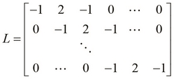
We can concisely define the matrix L using the following compute-matrix function. Note that for a given size n, we generate a matrix of size  :
:
(defn lmatrix [n]
  (compute-matrix :clatrix [n (+ n 2)]
                  (fn [i j] ({0 -1, 1 2, 2 -1} (- j i) 0))))
The anonymous closure in the preceding example uses a map to decide the value of an element at a specified row and column index. For example, the element at row index 2 and column index 3 is 2, since (- j i) is 1 and the key 1 in the map has 2 as its value. We can verify that the generated matrix has a similar structure as that of the matrix lmatrix through the REPL as follows:
user> (pm (lmatrix 4))
[[-1.000 2.000 -1.000  0.000  0.000  0.000]
[ 0.000 -1.000  2.000 -1.000  0.000  0.000]
[ 0.000  0.000 -1.000  2.000 -1.000  0.000]
[ 0.000  0.000  0.000 -1.000  2.000 -1.000]]
nil
Next, we define how to represent the data points that we intend to interpolate over. Each point has an observed value x that is passed to some function to produce another observed value y. For this example, we simply choose a random value for x and another random value for y. We perform this repeatedly to produce the data points.
In order to represent the data points along with an L matrix of compatible size, we define the following simple function named problem that returns a map of the problem definition. This comprises the L matrix, the observed values for x, the hidden values of x for which we have to estimate values of y to create a curve, and the observed values for y.
(defn problem
  "Return a map of the problem setup for a
  given matrix size, number of observed values
  and regularization parameter"
  [n n-observed lambda]
  (let [i (shuffle (range n))]
    {:L (M/* (lmatrix n) lambda)
     :observed (take n-observed i)
     :hidden (drop n-observed i)
     :observed-values (matrix :clatrix
                              (repeatedly n-observed rand))}))
The first two parameters of the function are the number of rows n in the L matrix, and the number of observed x values n-observed. The function takes a third argument lambda, which is actually the regularization parameter for our model. This parameter determines how accurate the estimated curve is, and we shall study more about how it's relevant to this model in the later chapters. In the map returned by the preceding function, the observed values for x and y have keys :observed and :observed-values, and the hidden values for x have the key :hidden. Similarly, the key :L is mapped to an L matrix of compatible size.
Now that we've defined our problem (or model), we can plot a smooth curve over the given points. By smooth, we mean that each point in the curve is the average of its immediate neighbors, along with some Gaussian noise. Thus, all the points on the curve of this noise have a Gaussian distribution, in which all the values are scattered about some mean value along with a spread specified by some standard deviation.
If we partition matrix L into  and
and  over the observed and hidden points respectively, we can define a formula to determine the curve as follows. The following equation may seem a bit daunting, but as mentioned earlier, we shall study the reasoning behind this equation in the following chapters. The curve can be represented by a matrix that can be calculated as follows, using the matrix L:
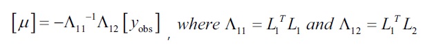
We estimate the observed values for the hidden values of x as  , using the originally observed values of y, that is,
  and the two matrices that are calculated from the interpolation matrix L. These two matrices are calculated using only the transpose and inverse functions of a matrix. As all the values on the right-hand side of this equation are either matrices or vectors, we use matrix multiplication to find the product of these values.
The previous equation can be implemented using the functions that we've explored earlier. In fact, the code comprises just this equation written as a prefix expression for the map returned by the problem function that we defined previously. We now define the following function to solve the problem returned by the problem function:
(defn solve
  "Return a map containing the approximated value
y of each hidden point x"
  [{:keys [L observed hidden observed-values] :as problem}]
  (let [nc  (column-count L)
        nr  (row-count L)
        L1  (cl/get L (range nr) hidden)
        L2  (cl/get L (range nr) observed)
        l11 (M/* (transpose L1) L1)
        l12 (M/* (transpose L1) L2)]
    (assoc problem :hidden-values
      (M/* -1 (inverse l11) l12 observed-values))))
The preceding function calculates the estimated values for y and simply adds them to the original map with the key :hidden-values using the assoc function.
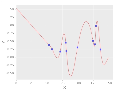
It's rather difficult to mentally visualize the calculated values of the curve, so we will now use the Incanter library (http://github.com/liebke/incanter) to plot the estimated curve and the original points. This library essentially provides a simple and idiomatic API to create and view various types of plots and charts.
Note
The Incanter library can be added to a Leiningen project by adding the following dependency to the project.clj file:
[incanter "1.5.4"]
For the upcoming example, the namespace declaration should look similar to the following:
(ns my-namespace
  (:use [incanter.charts :only [xy-plot add-points]]
        [incanter.core   :only [view]])
  (:require [clojure.core.matrix.operators :as M]
            [clatrix.core :as cl]))
We now define a simple function that will plot a graph of the given data using functions, such as xy-plot and view, from the Incanter library:
(defn plot-points
  "Plots sample points of a solution s"
  [s]
  (let [X (concat (:hidden s) (:observed s))
        Y (concat (:hidden-values s) (:observed-values s))]
    (view
     (add-points
      (xy-plot X Y) (:observed s) (:observed-values s)))))
As this is our first encounter with the Incanter library, let's discuss some of the functions that are used to implement plot-points. We first bind all the values on the x axis to X, and all values on the y axis to Y. Then, we plot the points as a curve using the xy-plot function, which takes two sets of values to plot on the x and y axes as arguments and returns a chart or plot. Next, we add the originally observed points to the plot using the add-points function. The add-points function requires three arguments: the original plot, a vector of all the values of the x axis component, and a vector of all the values of the y axis component. This function also returns a plot such as the xy-plot function, and we can view this plot using the view function. Note that we could have equivalently used the thread macro (->) to compose the xy-plot, add-points, and view functions.
Now, we can intuitively visualize the estimated curve using the plot-points function on some random data as shown in the following function:
(defn plot-rand-sample []
  (plot-points (solve (problem 150 10 30))))
When we execute the plot-rand-sample function, the following plot of the values is displayed: