
Probabilistic graphical models, seen from the point of view of mathematics, are a way to represent a probability distribution over several variables, which is called a joint probability distribution. In other words, it is a tool to represent numerical beliefs in the joint occurrence of several variables. Seen like this, it looks simple, but what PGM addresses is the representation of these kinds of probability distribution over many variables. In some cases, many could be really a lot, such as thousands to millions. In this section, we will review the basic notions that are fundamental to PGMs and see their basic implementation in R. If you're already familiar with these, you can easily skip this section. We start by asking why probabilities are a good tool to represent one's belief about facts and events, then we will explore the basics of probability calculus. Next we will introduce the fundamental building blocks of any Bayesian model and do a few simple yet interesting computations. Finally, we will speak about the main topic of this book: Bayesian inference.
Did I say Bayesian inference was the main topic before? Indeed, probabilistic graphical models are also a state-of-the-art approach to performing Bayesian inference or in other words to computing new facts and conclusions from your previous beliefs and supplying new data.
This principle of updating a probabilistic model was first discovered by Thomas Bayes and publish by his friend Richard Price in 1763 in the now famous An Essay toward solving a Problem in the Doctrine of Chances.
Probability theory is nothing but common sense reduced to calculation | ||
| --Théorie analytique des probabilités,1821. Pierre-Simon, marquis de Laplace | ||
As Pierre-Simon Laplace was saying, probabilities are a tool to quantify our common-sense reasoning and our degree of belief. It is interesting to note that, in the context of machine learning, this concept of belief has been somehow extended to the machine, that is, to the computer. Through the use of algorithms, the computer will represent its belief about certain facts and events with probabilities.
So let's take a simple example that everyone knows: the game of flipping a coin. What's the probability or the chance that coin will land on a head, or on a tail? Everyone should and will answer, with reason, a 50% chance or a probability of 0.5 (remember, probabilities are numbered between 0 and 1).
This simple notion has two interpretations. One we will call a frequentist interpretation and the other one a Bayesian interpretation. The first one, the frequentist, means that, if we flip the coin many times, in the long term it will land heads-up half of the time and tails-up the other half of the time. Using numbers, it will have a 50% chance of landing on one side, or a probability of 0.5. However, this frequentist concept, as the name suggests, is valid only if one can repeat the experiment a very large number of times. Indeed, it would not make any sense to talk about frequency if you observe a fact only once or twice. The Bayesian interpretation, on the other hand, quantifies our uncertainty about a fact or an event by assigning a number (between 0 and 1, or 0% and 100%) to it. If you flip a coin, even before playing, I'm sure you will assign a 50% chance to each face. If you watch a horse race with 10 horses and you know nothing about the horses and their rides, you will certainly assign a probability of 0.1 (or 10%) to each horse.
Flipping a coin is an experiment you can do many times, thousands of times or more if you want. However, a horse race is not an experiment you can repeat numerous times. And what is the probability your favorite team will win the next football game? It is certainly not an experiment you can do many times: in fact you will do it once, because there is only one match. But because you strongly believe your team is the best this year, you will assign a probability of, say, 0.9 that your team will win the next game.
The main advantage of the Bayesian interpretation is that it does not use the notion of long-term frequency or repetition of the same experiment.
In machine learning, probabilities are the basic components of most of the systems and algorithms. You might want to know the probability that an e-mail you received is a spam (junk) e-mail. You want to know the probability that the next customer on your online site will buy the same item as the previous customer (and whether your website should advertise it right away). You want to know the probability that, next month, your shop will have as many customers as this month.
As you can see with these examples, the line between purely frequentist and purely Bayesian is far from being clear. And the good news is that the rules of probability calculus are rigorously the same, whatever interpretation you choose (or not).
A central theme in machine learning and especially in probabilistic graphical models is the notion of a conditional probability. In fact, let's be clear, probabilistic graphical models are all about conditional probability. Let's get back to our horse race example. We say that, if you know nothing about the riders and their horses, you would assign, say, a probability of 0.1 to each (assuming there are 10 horses). Now, you just learned that the best rider in the country is participating in this race. Would you give him the same chance as the others? Certainly not! Therefore the probability for this rider to win is, say, 19% and therefore, we will say that all other riders have a probability to win of only 9%. This is a conditional probability: that is, a probability of an event based on knowing the outcome of another event. This notion of probability matches perfectly changing our minds intuitively or updating our beliefs (in more technical terms) given a new piece of information. At the same time we also saw a simple example of Bayesian update where we reconsidered and updated our beliefs given a new fact. Probabilistic graphical models are all about that but just with more complex situations.
In the previous section we saw why probabilities are a good tool to represent uncertainty or the beliefs and frequency of an event or a fact. We also mentioned the fact that the same rules of calculus apply for both the Bayesian and the frequentist interpretation. In this section, we will have a first look at the basic probability rules of calculus, and introduce the notion of a random variable which is central to Bayesian reasoning and the probabilistic graphical models.
In this section we introduce the basic concepts and the language used in probability theory that we will use throughout the book. If you already know those concepts, you can skip this section.
A sample space Ω is the set of all possible outcomes of an experiment. In this set, we call ω a point of Ω, a realization. And finally we call a subset of Ω an event.
For example, if we toss a coin once, we can have heads (H) or tails (T). We say that the sample space is  . An event could be I get a head (H). If we toss the coin twice, the sample space is bigger and we can have all those possibilities
  . An event could be I get a head first. Therefore my event is
  .
.
A more advanced example could be the measurement of someone's height in centimeters. The sample space is all the positive numbers from 0.0 to 10.9. Chances are that none of your friends will be 10.9 meters tall, but it does no harm to the theory. An event could be all the basketball players, that is, measurements that are 2 meters or more. In mathematical notation we write in terms of intervals  and
and 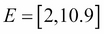 .
.
A probability is a real number Pr(E) that we assign to every event E. A probability must satisfy the three following axioms. Before writing them, it is time to recall why we're using these axioms. If you remember, we said that, whatever the interpretation of the probabilities that we make (frequentist or Bayesian), the rules governing the calculus of probability are the same:
-
For every event E,
 : we just say that probability is always positive
  , which means that the probability of having any of all the possible events is always 1. Therefore, from axiom 1 and 2, any probability is always between 0 and 1.
-
If you have independent events E1, E2, … then
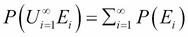 .
.
In a computer program, a variable is a name or a label associated to a storage space somewhere in the computer's memory. A program's variable is therefore defined by its location (and in many languages its type) and holds one and only one value. The value can be complex like an array or a data structure. The most important thing is that, at any time, the value is well known and not subject to change unless someone decides to change it. In other words, the value can only change if the algorithm using it changes it.
A random variable is something different: it is a function from a sample space into real numbers. For example, in some experiments, random variables are implicitly used:
When throwing two dices, X is the sum of the numbers is a random variable
When tossing a coin N times, X is the number of heads in N tosses is a random variable
For each possible event, we can associate a probability pi and the set of all those probabilities is the probability distribution of the random variable.
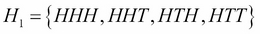
Let's see an example: we consider an experiment in which we toss a coin three times. A sample point (from the sample space) is the result of the three tosses. For example, HHT, two heads and one tail, is a sample point.
Therefore, it is easy to enumerate all the possible outcomes and find that the sample space is:

Let's Hi be the event that the ith toss is a head. So for example:
If we assign a probability of  to each sample point, then using enumeration we see that
 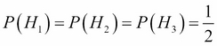 .
.
Under this probability model, the events H1, H2, H3 are mutually independent. To verify, we first write that:

We must also check each pair. For example:
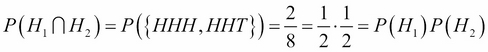
The same applies to the two other pairs. Therefore H1, H2, H3 are mutually independent. In general, we write that the probability of two independent events is the product of their probability:  . And we write that the probability of two disjoint independent events is the sum of their probability:
  .
.
If we consider a different outcome, we can define another probability distribution. For example, let's consider again the experiment in which a coin is tossed three times. This time we consider the random variable X as the number of heads obtained after three tosses.
A complete enumeration gives the same sample space as before:
But as we consider the number of heads, the random variable X will map the sample space to the following numbers this time:
|
s |
HHH |
HHT |
HTH |
THH |
TTH |
THT |
HTT |
TTT |
|---|---|---|---|---|---|---|---|---|
|
X(s) |
3 |
2 |
2 |
2 |
1 |
1 |
1 |
0 |
So the range for the random variable X is now {0,1,2,3}. If we assume the same probability for all points as before, that is , then we can deduce the probability function on the range of X:
|
x |
0 |
1 |
2 |
3 |
|---|---|---|---|---|
|
P(X=x) |
|
 |
|
|
Let's come back to the first game: 2 heads and a 6 simultaneously, the hard game with a low probability of winning. We can associate to the coin toss experiment a random variable N, which is the number of heads after two tosses. This random variable summarizes our experiment very well and N can take the values 0, 1, or 2. So instead of saying we're interested in the event of having two heads, we can say equivalently that we are interested in the event N=2. This approach allows us to look at other events, such as having only one head (HT or TH) and even having zero heads (TT). We say that the function assigning a probability to each value of N is called a probability distribution. Another random variable is D, the number we obtain when we throw a dice.
When we consider the two experiments together (tossing a coin twice and throwing a dice), we are interested in the probability of obtaining either 0, 1, or 2 heads and at the same time obtaining either 1, 2, 3, 4, 5, or 6 with the dice. The probability distribution of these two random variables considered at the same time is written P(N, D) and it is called a joint probability distribution.
If we keep adding more and more experiments and therefore more and more variables, we can write a very big and complex joint probability distribution. For example, I could be interested in the probability that it will rain tomorrow, that the stock market will rise and that there will be a traffic jam on the highway that I take to go to work. It's a complex one but not unrealistic. I'm almost sure that the stock market and the weather are really not dependent. However, the traffic condition and the weather are seriously connected. I would like to write the distribution P(W, M, T)—weather, market, traffic—but it seems to be overly complex. In fact, it is not and this is what we will see throughout this book.
A probabilistic graphical model is a joint probability distribution. And nothing else.
One last and very important notion regarding joint probability distributions is marginalization. When you have a probability distribution over several random variables, that is a joint probability distribution, you may want to eliminate some of the variables from this distribution to have a distribution on fewer variables. This operation is very important. The marginal distribution p(X) of a joint distribution p(X, Y) is obtained by the following operation:
 where we sum the probabilities over all the possible values of y. By doing so, you can eliminate Y from P(X, Y). As an exercise, I'll let you think about the link between this and the probability of two disjoint events that we saw earlier.
For the math-orientated readers, when Y is a continuous variable, the marginalization can be written as 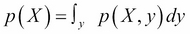 .
.
This operation is extremely important and hard to compute for probabilistic graphical models and most if not all the algorithms for PGM try to propose an efficient solution to this problem. Thanks to these algorithms, we can do complex yet efficient models on many variables with real-world data.
Let's continue our exploration of the basic concepts we need to play with probabilistic graphical models. We saw the notion of marginalization, which is important because, when you have a complex model, you may want to extract information about one or a few variables of interest. And this is when marginalization is used.
But the two most important concepts are conditional probability and Bayes' rule.
A conditional probability is the probability of an event conditioned on the knowledge of another event. Obviously, the two events must be somehow dependent otherwise knowing one will not change anything for the other:
What's the probability of rain tomorrow? And what's the probability of a traffic jam in the streets?
Knowing it's going to rain tomorrow, what is now the probability of a traffic jam? Presumably higher than if you knew nothing.
This is a conditional probability. In more formal terms, we can write the following formula:
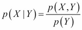 and
and 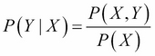
From these two equations we can easily deduce the Bayes formula:
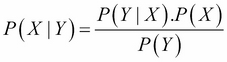
This formula is the most important and it helps invert probabilistic relationships. This is the chef d'oeuvre of Laplace's career and one of the most important formulas in modern science. Yet it is very simple.
In this formula, we call P(X | Y) the posterior distribution of X given Y. Therefore, we also call P(X) the prior distribution. We also call P(Y | X) the likelihood and finally P(Y) is the normalization factor.
The normalization factor needs a bit of explanation and development here. Recall that 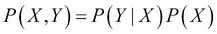 . And also, we saw that
 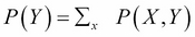 , an operation we called marginalization, whose goal was to eliminate (or marginalize out) a variable from a joint probability distribution.
So from there, we can write  .
.
Thanks to this magic bit of simple algebra, we can rewrite the Bayes' formula in its general form and also the most convenient one:
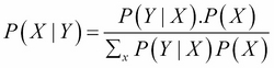
The simple beauty of this form is that we only need to specify and use P(Y |X) and P(X), that is, the prior and likelihood. Despite the simple form, the sum in the denominator, as we will see in the rest of this book, can be a hard problem to solve and advanced techniques will be required for advanced problems.
Now that we saw the famous formula with X and Y, two random variables, let me rewrite it with two other variables. After all, the letters are not important but it can shed some light on the intuition behind this formula:
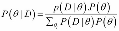
The intuition behind these concepts is the following:
The prior distribution P(θ) is what I believe about X before everything else is known—my initial belief.
The likelihood given a value for θ, what is the data D that I could generate, or in other terms what is the probability of D for all values of θ?
The posterior distribution P(θ | D) is finally the new belief I have about θ given some data D I observed.
This formula also gives the basis of a forward process to update my beliefs about the variable θ. Applying Bayes' rule will calculate the new distribution of θ. And if I receive new information again, I can update my beliefs again, and again.
In this section we will look at our first Bayesian program in R. We will define discrete random variables, that is, random variables that can only take a predefined number of values. Let's say we have a machine that makes light bulbs. You want to know if the machine works as planned or if it's broken. In order to do that you can test each bulb but that would be too many bulbs to test. With only a few samples and Bayes' rule you can estimate if the machine is correctly working or not.
When building a Bayesian model, we need to always set up the two main components:
The prior distribution
The likelihood
In this example, we won't need a specific package; we just need to write a simple function to implement a simple form of the Bayes' rule.
The prior distribution is our initial belief on how the machine is working or not. We identified a first random variable M for the state of the machine. This random variable can have two states {working, broken}. We believe our machine is working well because it's a good machine, so let's say the prior distribution is as follows:
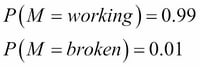
It simply says that our belief that the machine is working is really high, with a probability of 99% and only a 1% chance that it is broken. Here, clearly we're using the Bayesian interpretation of probability because we don't have many machines but just one. We could also ask the machine's vendor about the frequency of working machines he or she is able to produce. And we could use his or her number and, in that case, this probability would have a frequentist interpretation. Nevertheless, the Bayes' rule works in all the cases.
The second random variable is L and it is the light bulb produced by the machine. The light bulb can either be good or bad. So this random variable will have two states again {good, bad}.
Again, we need to give a prior distribution for the light bulb variable L: in the Bayes' formula, it is required that we specify a prior distribution and the likelihood distribution. In this case, the likelihood is P(L | M) and not simply P(L).
Here we need in fact to define two probability distributions: one when the machine works M = working and one when the machine is broken M = broken. And we ask the question twice:
How likely is it to have a good or a bad light bulb when the machine is working?
How likely is it to have a good or a bad light bulb when the machine is not working?
Let's try to give our best guess, either Bayesian or frequentist, because we have some statistics:
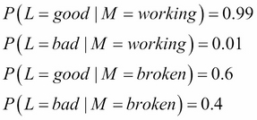
Here we believe that, if the machine is working, it will only give one bad light bulb out of 100, which is even higher than what we said before. But in this case, we know that the machine is working so we expect a very high success rate. However, if the machine is broken, we say we expect at least 40% of the light bulbs to be bad. From now on, we have fully specified our model and we can start using it.
Using a Bayesian model is to compute posterior distributions when a new fact is available. In our case, we want to know if the machine is working knowing that we just observed that our latest light bulb was not working. So we want to compute P(M | L). We just specified P(M) and P(L | M), so the last thing we have to do is to use the Bayes' formula to invert the probability distribution.
For example, let's say the last produced light bulb is bad, that is, L = bad. Using the Bayes formula we obtain:
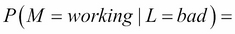
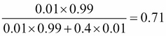
Or if you prefer, a 71% chance that the machine is working. It's lower but follows our intuition that the machine might still work. After all even if we received a bad light bulb, it's only one and maybe the next will still be good.
Let's try to redo the same problem, with equal priors on the state of the machine: a 50% chance the machine is working and 50% the machine is broken. The result is therefore:
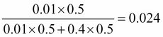
It is a 2.4% chance the machine is working! That's very low. Indeed, given the apparent quality of this machine, as modeled in the likelihood, it appears very surprising that the machine can produce a bad light bulb. In this case, we didn't make the assumption that the machine was working as in the previous example, and having a bad light bulb can be seen as an indication that something is wrong.
After seeing this previous example, the first legitimate question one can ask is what we would do if we observed more than one light bulb. Indeed, it seems a bit strange to conclude that the machine needs to be repaired only after seeing one bad light bulb. The Bayesian way to do it is to use the posterior as the new prior and update the posterior distribution in sequence. As it would be a bit onerous to do that by hand, we will write our first Bayesian program in R.
The following code is a function that computes the posterior distribution of a random variable given the prior distribution and the likelihood and a sequence of observed data. This function takes three arguments: the prior distribution, the likelihood, and a sequence of data. The prior and data are a vector and the likelihood a matrix:
prior <- c(working = 0.99, broken = 0.01)
likelihood <- rbind(
    working = c(good=0.99, bad=0.01), broken = c(good=0.6, bad=0.4))
data <- c("bad","bad","bad","bad")
So we defined three variables, the prior with two states working and broken, the likelihood we specified for each condition of the machine (working or broken), and the distribution over the variable L of the light bulb. So that's four values in total and the R matrix is indeed like the conditional distribution we defined in the previous section:
likelihood
          good    bad
working   0.99    0.01
broken    0.60    0.40
The data variable contains the sequence of observed light bulbs we will use to test our machine and compute the posterior probabilities. So, now we can define our Bayesian update function as follows:
bayes <- function(prior, likelihood, data)
{
  posterior <- matrix(0, nrow=length(data), ncol=length(prior))
  dimnames(posterior) <- list(data, names(prior))

  initial_prior <- prior
  for(i in 1:length(data))
  {
    posterior[i, ] <-
      prior*likelihood[ , data[i]]/
      sum(prior * likelihood[ , data[i]])

    prior <- posterior[i , ]
  }

  return(rbind(initial_prior,posterior))
}
This function does the following:
It creates a matrix to store the results of the successive computation of the posterior distributions
Then for each data it computes the posterior distribution given the current prior: you can see the Bayes formula in the R code, exactly as we saw it earlier
Finally, the new prior is the current posterior and the same process can be re-iterated
In the end, the function returns a matrix with the initial prior and all subsequent posterior distributions.
Let's do a few runs to understand how it works. We will use the function matplot to draw the evolution of the two distributions, one for the posterior probability that the machine is working (in green) and the other in red, meaning that the machine is broken:
matplot( bayes(prior,likelihood,data), t='b', lty=1, pch=20, col=c(3,2))
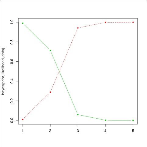
The result can be seen on the following graph: as the bad light bulbs arrive, the probability that the machine will fail quickly falls (the plain or green line). We expected something like 1 bad light bulb out of 100, and not that many. So this machine needs maintenance now. The red or dashed line represents the probability that the machine is broken.
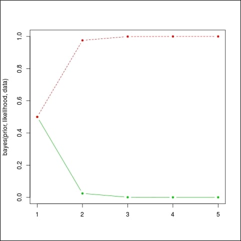
If the prior was different, we would have seen a different evolution. For example, let's say that we have no idea if the machine is broken or not, that is, we give an equal chance to each situation:
prior <- c(working = 0.5, broken = 0.5)
Run the code again:
matplot( bayes(prior,likelihood,data), t='b', lty=1, pch=20, col=c(3,2))
Again we obtain a quick convergence to very high probabilities that the machine is broken, which is not surprising given the long sequence of bad light bulbs:
If we keep playing with the data we might see different behaviors again. For example, let's say we assume the machine is working well, with a 99% probability. And we observe a sequence of 10 light bulbs, among which the first one is bad. In R we have:
prior=c(working=0.99,broken=0.01)
data=c("bad","good","good","good","good","good","good","good","good","good")
matplot(bayes(prior,likelihood,data),t='b',pch=20,col=c(3,2))
And the result is given in the following graph:
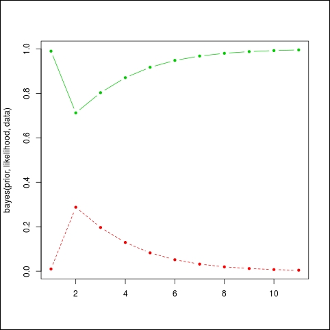
The algorithm hesitates at first because, given such a good machine, it's unlikely to see a bad light bulb, but then it will converge back to high probabilities again, because the sequence of good light bulbs does not indicate any problem.
This concludes our first example of a Bayesian model with R. In the rest of this chapter, we will see how to create real-world models, with more than just two very simple random variables, and how to solve two important problems:
The problem of inference, which is the problem of computing the posterior distribution when we receive new data
The problem of learning, which is the determination of prior probabilities from a dataset
A careful reader should now ask: doesn't this little algorithm we just saw solve the problem of inference? Indeed it does, but only when one has two discrete variables, which is a bit too simple to capture the complexity of the world. We will introduce now the core of this book and the main tool for performing Bayesian inference: probabilistic graphical models.