
Unsupervised learning is about analyzing the data and discovering hidden structures in unlabeled data. As no notion of the right labels is given, there is also no error measure to evaluate a learned model; however, unsupervised learning is an extremely powerful tool. Have you ever wondered how Amazon can predict what books you'll like? How Netflix knows what you want to watch before you do? The answer can be found in unsupervised learning. The following is one such example.
Many problems can be formulated as finding similar sets of elements, for example, customers who purchased similar products, web pages with similar content, images with similar objects, users who visited similar websites, and so on.
Two items are considered similar if they are a small distance apart. The main questions are how each item is represented and how is the distance between the items defined. There are two main classes of distance measures: Euclidean distances and non-Euclidean distances.
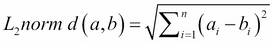
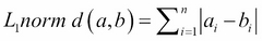
In the Euclidean space, with the n dimension, the distance between two elements is based on the locations of the elements in such a space, which is expressed as p-norm distance. Two commonly used distance measures are L2 and L1 norm distances.
L2 norm, also known as Euclidean distance, is the most frequently applied distance measure that measures how far apart two items in a two-dimensional space are. It is calculated as a square root of the sum of the squares of the differences between elements a and b in each dimension, as follows:
L1 norm, also known as Manhattan distance, city block distance, and taxicab norm, simply sums the absolute differences in each dimension, as follows:
A non-Euclidean distance is based on the properties of the elements, but not on their location in space. Some well-known distances are Jaccard distance, cosine distance, edit distance, and Hamming distance.
Jaccard distance is used to compute the distance between two sets. First, we compute the Jaccard similarity of two sets as the size of their intersection divided by the size of their union, as follows:
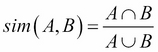
The Jaccard distance is then defined as 1 minus Jaccard similarity, as shown in the following:
Cosine distance between two vectors focuses on the orientation and not magnitude, therefore, two vectors with the same orientation have cosine similarity 1, while two perpendicular vectors have cosine similarity 0. Suppose we have two multidimensional points, think of a point as a vector from origin (0,0, …, 0) to its location. Two vectors make an angle, whose cosine distance is a normalized dot-product of the vectors, as follows:
Cosine distance is commonly used in a high-dimensional feature space; for instance, in text mining, where a text document represents an instance, features that correspond to different words, and their values corresponds to the number of times the word appears in the document. By computing cosine similarity, we can measure how likely two documents match in describing similar content.
Edit distance makes sense when we compare two strings. The distance between the a=a1a2a3…an and b=b1b2b3…bn strings is the smallest number of the insert/delete operation of single characters required to convert the string from a to b. For example, a = abcd and b = abbd. To convert a to b, we have to delete the second b and insert c in its place. No smallest number of operations would convert a to b, thus the distance is d(a, b)=2.
Hamming distance compares two vectors of the same size and counts the number of dimensions in which they differ. In other words, it measures the number of substitutions required to convert one vector into another.
There are many distance measures focusing on various properties, for instance, correlation measures the linear relationship between two elements: Mahalanobis distance that measures the distance between a point and distribution of other points and SimRank, which is based on graph theory, measures similarity of the structure in which elements occur, and so on. As you can already imagine selecting and designing the right similarity measure for your problem is more than half of the battle. An impressive overview and evaluation of similarity measures is collected in Chapter 2, Similarity and Dissimilarity Measures in the book Image Registration: Principles, Tools and Methods by A. A. Goshtasby (2012).
The curse of dimensionality refers to a situation where we have a large number of features, often hundreds or thousands, which lead to an extremely large space with sparse data and, consequently, to distance anomalies. For instance, in high dimensions, almost all pairs of points are equally distant from each other; in fact, almost all the pairs have distance close to the average distance. Another manifestation of the curse is that any two vectors are almost orthogonal, which means all the angles are close to 90 degrees. This practically makes any distance measure useless.
A cure for the curse of dimensionality might be found in one of the data reduction techniques, where we want to reduce the number of features; for instance, we can run a feature selection algorithm such as ReliefF or feature extraction/reduction algorithm such as PCA.
Clustering is a technique for grouping similar instances into clusters according to some distance measure. The main idea is to put instances that are similar (that is, close to each other) into the same cluster, while keeping the dissimilar points (that is, the ones further apart from each other) in different clusters. An example of how clusters might look is shown in the following diagram:
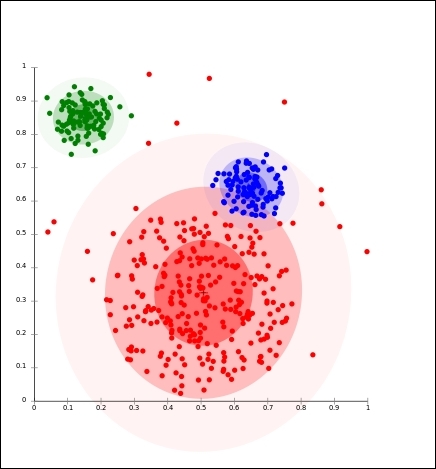
The clustering algorithms follow two fundamentally different approaches. The first is a hierarchical or agglomerative approach that first considers each point as its own cluster, and then iteratively merges the most similar clusters together. It stops when further merging reaches a predefined number of clusters or if the clusters to be merged are spread over a large region.
The other approach is based on point assignment. First, initial cluster centers (that is, centroids) are estimated—for instance, randomly—and then, each point is assigned to the closest cluster, until all the points are assigned. The most well-known algorithm in this group is k-means clustering.
The k-means clustering picks initial cluster centers either as points that are as far as possible from one another or (hierarchically) clusters a sample of data and picks a point that is the closest to the center of each of the k clusters.