
The road to the mastery of Tableau begins with three essential concepts. We will consider each of the following in turn:
Dimensions and measures
Row level, aggregate level, and table level
Continuous and discrete
Tableau categorizes every field from an underlying data source as either a dimension or a measure. A dimension is qualitative or, to use another word, categorical. A measure is quantitative or aggregable. A measure is usually a number but may be an aggregated, non-numeric field, such as MAX(Order Date). A dimension is usually a text, Boolean, or date field, but may also be a number, such as Order_ID. Dimensions provide meaning to numbers by slicing those numbers into separate parts/categories. Measures without dimensions are mostly meaningless.
Let's consider an example to better understand this concept.
In the workbook associated with this chapter, navigate to the worksheet entitled
Dimensions and Measures.Drag Sales to the Rows shelf.
Place Order Date and Category on the Columns shelf:

The result of step 2 is mostly meaningless. The measure Sales is about $2.3 million, but without the context supplied by slicing the measure with one or more dimensions, there is no way to understand what it means. Step 2 brings meaning. Placing Order Date and Category on the Columns shelf provides context, which imparts meaning to the visualization.
There are three levels of calculations in Tableau: Row, Aggregate, and Table. To understand how these three levels function, it is important to be familiar with the Tableau process flow:
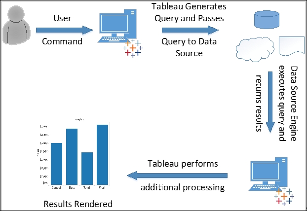
Let's follow the flow of the preceding figure to understand where the three levels of calculations take place. We will do so via an example considering the fields Profit and Sales. Assuming SQL, consider the following calculation types, calculated fields, and queries. Note that the SQL is simplified for the sake of the example:
|
Calculation type |
Calculated field in Tableau |
Query passed to Data Source |
|
Row level |
|
|
|
Aggregate level |
|
|
|
Table level |
|
|
For the row-level calculation, the computation is actually completed by the data-source engine. Tableau merely displays the results. For the aggregate level calculation, Tableau does a little bit more than display the results; it also divides the two numbers that are returned by the data-source engine. For the table-level calculation, Tableau may perform additional computations on the returned results. Let's explore further via an exercise using the similar calculated fields.
In the workbook associated with this chapter, navigate to the worksheet entitled
Row_Agg_Tbl.Navigate to Analysis | Create Calculated Field to create the following calculated fields. Note that each must be created separately; it is not possible in this context to create a single calculated field containing all three calculations:
Name
Calculation
Lev - Row
[Number of Records]/[Quantity]Lev - Agg
SUM([Number of Records])/SUM(Quantity)Lev - Tab
WINDOW_AVG([Lev - Agg])In the Data pane, right-click on the three calculated fields you just created and navigate to Default Properties | Number format.
In the resulting dialog box, select Percentage and click OK.
Place Order Date on the Columns shelf.
Place Measure Names on the Rows shelf and Measure Values on the Text shelf.
Exclude all values except for Lev - Row, Lev - Agg, and Lev - Tab:

Lev - Agg is an aggregate-level calculation. The aggregated results of [Number of Records] and [Quantity] are returned by the data-source engine. Tableau divides those results and displays values for each year.
Lev - Row is a row-level calculation. The computation is completed by the data-source engine. [Number of Records] is divided by [Quantity] for each row of the underlying data. The results are then summed across all rows. Of course, in this case, the row-level calculation does not provide useful results; however, since a new Tableau author may mistakenly create a row-level calculation when an aggregate-level calculation is what is really needed, the example is included here.
Lev - Tab is a table-level calculation. Some of the computation is completed by the data-source engine; that is, the aggregation. Tableau completes additional computation on the results returned from the data-source engine. Specifically, the results of Lev - Agg are summed and then divided by the number of members in the dimension. For the preceding example, this is (26.29% + 26.34% + 26.30% + 26.55%)/4. Once again, the results in this case are not particularly helpful, but they do demonstrate knowledge the budding Tableau author should possess.
Continuous and discrete are not concepts that are unique to Tableau. Indeed, both can be observed in many arenas. Consider the following example:
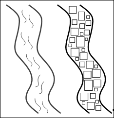
This is an image of two rivers - River-Left and River-Right. Water is flowing in River-Left. River-Right is composed of ice cubes. Could you theoretically sort the ice cubes in River-Right? Yes! Is there any way to sort the water in River-Left? In other words, could you take buckets of water from the bottom of the river, cart those buckets upstream and pour the water back into River-Left and thereby say, I have sorted the water in the river? No. The H2O in River-Left is in continuous form; that is, water. The H2O in River-Right is in discrete form; that is, ice.
Having considered an example of continuous and discrete in natural phenomena, let's turn our attention back to Tableau. Continuous and discrete in Tableau can be more clearly understood via the following seven considerations:
Continuous is green. Discrete is blue. Select any field in the Data pane or place any field on a shelf and you will note that it is either green or blue. Also, the icons associated with fields are either green or blue.
Continuous is always numeric. Discrete may be a string.
Continuous and discrete are not synonymous with dimension and measure. It is common for new Tableau authors to confuse continuous with measure and discrete with dimension. They are not synonymous. A measure may be either discrete or continuous. Also, a dimension, if it is a number, may be discrete or continuous. To prove the point, right-click on any numeric or date field in Tableau and note that you can convert it:

Discrete is sortable. Continuous is not sortable. Sortable/not sortable behavior is most easily observed with dates, as shown in the following screenshot:

Continuous colors are gradients. Discrete colors are distinct. The following example shows Profit as continuous and then as discrete. Note the difference in how colors are rendered. The left portion of the following screenshot demonstrates that continuous results in gradients and the right portion demonstrates that discrete results in distinct colors:

Continuous pills can be placed to the right of discrete pills, but not to the left. In the following screenshot, note that the Tableau author can place Region to the right of Year when Year is discrete. Further note that the Tableau author is unable to place Region to the right of Year when Year is continuous:

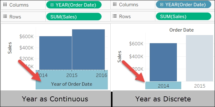
Continuous creates axes. Discrete creates headers. Note that in the left portion of the following screenshot, Year(Order Date) is continuous and the Year of Order Date axis is selected. Since Year of Order Date is an axis, the entire x-plane is selected. In the right portion of the screenshot, Year(Order Date) is discrete and 2014 is selected. Since 2014 is a header, only it is selected and not the entire x-plane: