
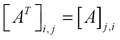
Another frequently used elementary matrix operation is the transpose of a matrix. The transpose of a matrix A is represented as  or
or  . A simple way to define the transpose of a matrix is by reflecting the matrix over its prime diagonal. By prime diagonal, we mean the diagonal comprising elements whose row and column indices are equal. We can also describe the transpose of a matrix by swapping of the rows and columns of a matrix. We can use the following
 transpose function from core.matrix to perform this operation:
user> (def A (matrix [[1 2 3] [4 5 6]]))
#'user/A
user> (pm (transpose A))
[[1.000 4.000]
 [2.000 5.000]
 [3.000 6.000]]
nil
We can define the following three possible ways to obtain the transpose of a matrix:
The original matrix is reflected over its main diagonal
The rows of the matrix become the columns of its transpose
The columns of the matrix become the rows of its transpose
Hence, every element in a matrix has its row and column swapped in its transpose, and vice versa. This can be formally represented using the following equation:
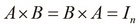
This brings us to the notion of an invertible matrix. A square matrix is said to be invertible if there exists another square matrix that is the inverse of a matrix, and which produces an identity matrix when multiplied with the original matrix. A matrix A of size  , is said to have an inverse matrix B if the following equality is true:
Let's test this equality using the inverse function from core.matrix. Note that the default persistent implementation of the core.matrix library does not implement the inverse operation, so we use a matrix from the clatrix library instead. In the following example, we create a matrix from the clatrix library using the cl/matrix function, determine its inverse using the inverse function, and multiply these two matrices using the M/* function:
user> (def A (cl/matrix [[2 0] [0 2]]))
#'user/A
user> (M/* (inverse A) A)
 A 2x2 matrix
 -------------
 1.00e+00  0.00e+00
 0.00e+00  1.00e+00
In the preceding example, we first define a matrix A and then multiply it with its inverse to produce the corresponding identity matrix. An interesting observation when we use double precision numeric types for the elements in a matrix is that not all matrices produce an identity matrix on multiplication with their inverse.
A small amount of error can be observed for some matrices, and this happens due to the limitations of using a 32-bit representation for floating-point numbers; this is shown as follows:
user> (def A (cl/matrix [[1 2] [3 4]]))
#'user/A
user> (inverse A)
 A 2x2 matrix
 -------------
-2.00e+00  1.00e+00
 1.50e+00 -5.00e-01
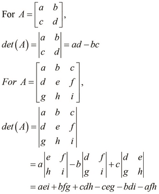
In order to find the inverse of a matrix, we must first define the determinant of that matrix, which is simply another value determined from a given matrix. First off, determinants only exist for square matrices, and thus, inverses only exist for matrices with an equal number of rows and columns. The determinant of a matrix is represented as  or
or  . A matrix whose determinant is zero is termed as a singular matrix. For a matrix A, we define its determinant as follows:
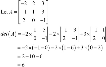
We can use the preceding definitions to express the determinant of a matrix of any size. An interesting observation is that the determinant of an identity matrix is always 1. As an example, we will find the determinant of a given matrix as follows:
For a  matrix, we can use Sarrus' rule as an alternative means to calculate the determinant of a matrix. To find the determinant of a matrix using this scheme, we first write out the first two columns of the matrix to the right of the third column, so that there are five columns in a row. Next, we add the products of the diagonals going from top to bottom, and subtract the products of diagonals from bottom. This process can be illustrated using the following diagram:
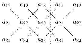
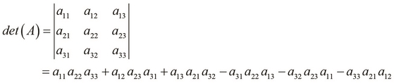
By using Sarrus' rule, we formally express the determinant of a matrix A as follows:
We can calculate the determinant of a matrix in the REPL using the following det function from core.matrix. Note that this operation is not implemented by the default persistent vector implementation of core.matrix.
user> (def A (cl/matrix [[-2 2 3] [-1 1 3] [2 0 -1]]))
#'user/A
user> (det A)
6.0
Now that we've defined the determinant of a matrix, let's use it to define the inverse of a matrix. We've already discussed the notion of an invertible matrix; finding the inverse of a matrix is simply determining a matrix such that it produces an identity matrix when multiplied with the original matrix.
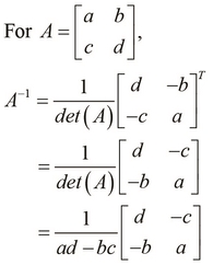
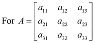
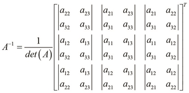
For the inverse of a matrix to exist, its determinant must be nonzero. Next, for each element in the original matrix, we find the determinant of the matrix without the row and column of the selected element. This produces a matrix of an identical size as that of the original matrix (termed as the cofactor matrix of the original matrix). The transpose of the cofactor matrix is called the adjoint of the original matrix. The adjoint produces the inverse on dividing it by the determinant of the original matrix. Now, let's formally define the inverse of a  matrix A. We denote the inverse of a matrix A as
  , and it can be formally expressed as follows:
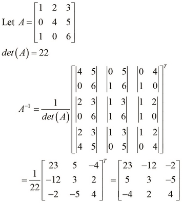
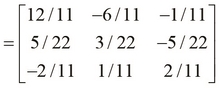
As an example, let's find the inverse of a sample matrix. We can actually verify that the inverse produces an identity matrix when multiplied with the original matrix, as shown in the following example:
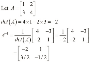
Similarly, we define the inverse of a matrix as follows:
Now, let's calculate the inverse of a matrix:
We've mentioned that singular and nonsquare matrices don't have inverses, and we can see that the inverse function throws an error when supplied with such a matrix. As shown in the following REPL output, the inverse function will throw an error if the given matrix is not a square matrix, or if the given matrix is singular:
user> (def A (cl/matrix [[1 2 3] [4 5 6]]))
#'user/A
user> (inverse A)
ExceptionInfo throw+: {:exception "Cannot invert a non-square matrix."}  clatrix.core/i (core.clj:1033)
user> (def A (cl/matrix [[2 0] [2 0]]))
#'user/A
user> (M/* (inverse A) A)
LapackException LAPACK DGESV: Linear equation cannot be solved because the matrix was singular.  org.jblas.SimpleBlas.gesv (SimpleBlas.java:274)