The scikit-learn library is organized into submodules. Each submodule contains algorithms and helper methods for a certain class of machine learning models and approaches.

Here is a sample of those submodules, including some example models:

While these approaches are diverse, a scikit-learn library abstracts away a lot of differences by exposing a regular interface to most of these algorithms. All of the example algorithms listed in the table implement a fit method, and most of them implement predict as well. These methods represent two phases in machine learning. First, the model is trained on the existing data with the fit method. Once trained, it is possible to use the model to predict the class or value of unseen data with predict. We will see both the methods at work in the next sections.

The scikit-learn library is part of the PyData ecosystem. Its codebase has seen steady growth over the past six years, and with over hundred contributors, it is one of the most active and popular among the scikit toolkits.

In contrast to the heterogeneous domains and applications of machine learning, the data representation in scikit-learn is less diverse, and the basic format that many algorithms expect is straightforward—a matrix of samples and features.

The underlying data structure is a numpy and the ndarray. Each row in the matrix corresponds to one sample and each column to the value of one feature.

There is something like Hello World in the world of machine learning datasets as well; for example, the Iris dataset whose origins date back to 1936. With the standard installation of scikit-learn, you already have access to a couple of datasets, including Iris that consists of 150 samples, each consisting of four measurements taken from three different Iris flower species:

>>> import numpy as np
>>> from sklearn import datasets
>>> iris = datasets.load_iris()

The dataset is packaged as a bunch, which is only a thin wrapper around a dictionary:

>>> type(iris)
sklearn.datasets.base.Bunch
>>> iris.keys()
['target_names', 'data', 'target', 'DESCR', 'feature_names']

Under the data key, we can find the matrix of samples and features, and can confirm its shape:

>>> type(iris.data)
numpy.ndarray
>>> iris.data.shape
(150, 4)

Each entry in the data matrix has been labeled, and these labels can be looked up in the target attribute:

>>> type(iris.target)
numpy.ndarray
>>> iris.target.shape
(150,)
>>> iris.target[:10]
array([0, 0, 0, 0, 0, 0, 0, 0, 0, 0])
>>> np.unique(iris.target)
array([0, 1, 2])

The target names are encoded. We can look up the corresponding names in the target_names attribute:

>>> iris.target_names
>>> array(['setosa', 'versicolor', 'virginica'], dtype='|S10')

This is the basic anatomy of many datasets, such as example data, target values, and target names.

What are the features of a single entry in this dataset?:

>>> iris.data[0]
array([ 5.1,  3.5,  1.4,  0.2])

The four features are the measurements taken of real flowers: their sepal length and width, and petal length and width. Three different species have been examined: the Iris-Setosa, Iris-Versicolour, and Iris-Virginica.

Machine learning tries to answer the following question: can we predict the species of the flower, given only the measurements of its sepal and petal length?

In the next section, we will see how to answer this question with scikit-learn.

Besides the data about flowers, there are a few other datasets included in the scikit-learn distribution, as follows:

A few datasets are not included, but they can easily be fetched on demand (as these are usually a bit bigger). Among these datasets, you can find a real estate dataset and a news corpus:

>>> ds = datasets.fetch_california_housing()
downloading Cal. housing from http://lib.stat.cmu.edu/modules.php?op=...
>>> ds.data.shape
(20640, 8)
>>> ds = datasets.fetch_20newsgroups()
>>> len(ds.data)
11314
>>> ds.data[0][:50]
u"From: [email protected] (where's my thing)\nSubjec"
>>> sum([len([w for w in sample.split()]) for sample in ds.data])
3252437

These datasets are a great way to get started with the scikit-learn library, and they will also help you to test your own algorithms. Finally, scikit-learn includes functions (prefixed with datasets.make_) to create artificial datasets as well.

If you work with your own datasets, you will have to bring them in a shape that scikit-learn expects, which can be a task of its own. Tools such as Pandas make this task much easier, and Pandas DataFrames can be exported to numpy.ndarray easily with the as_matrix() method on DataFrame.

In this section, we will show short examples for both classification and regression.

Classification problems are pervasive: document categorization, fraud detection, market segmentation in business intelligence, and protein function prediction in bioinformatics.

While it might be possible for hand-craft rules to assign a category or label to new data, it is faster to use algorithms to learn and generalize from the existing data.

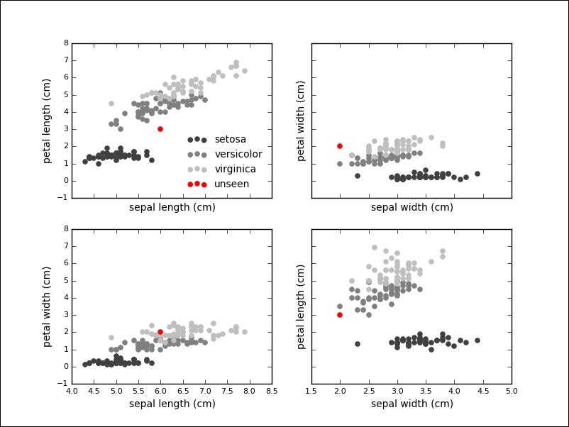
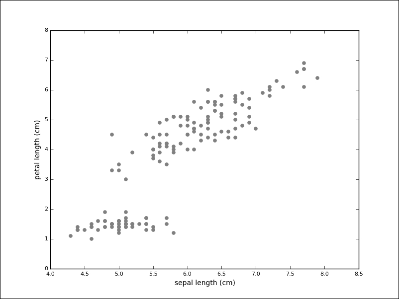
We will continue with the Iris dataset. Before we apply a learning algorithm, we want to get an intuition of the data by looking at some values and plots.

All measurements share the same dimension, which helps to visualize the variance in various boxplots:

We see that the petal length (the third feature) exhibits the biggest variance, which could indicate the importance of this feature during classification. It is also insightful to plot the data points in two dimensions, using one feature for each axis. Also, indeed, our previous observation reinforced that the petal length might be a good indicator to tell apart the various species. The Iris setosa also seems to be more easily separable than the other two species:

From the visualizations, we get an intuition of the solution to our problem. We will use a supervised method called a Support Vector Machine (SVM) to learn about a classifier for the Iris data. The API separates models and data, therefore, the first step is to instantiate the model. In this case, we pass an optional keyword parameter to be able to query the model for probabilities later:

>>> from sklearn.svm import SVC
>>> clf = SVC(probability=True)

The next step is to fit the model according to our training data:

>>> clf.fit(iris.data, iris.target)
SVC(C=1.0, cache_size=200, class_weight=None, coef0=0.0,
    degree=3, gamma=0.0, kernel='rbf', max_iter=-1,
    probability=True, random_state=None, shrinking=True,
    tol=0.001, verbose=False)

With this one line, we have trained our first machine learning model on a dataset. This model can now be used to predict the species of unknown data. If given some measurement that we have never seen before, we can use the predict method on the model:

>>> unseen = [6.0, 2.0, 3.0, 2.0]
>>> clf.predict(unseen)
array([1])
>>> iris.target_names[clf.predict(unseen)]
array(['versicolor'],
      dtype='|S10')

We see that the classifier has given the versicolor label to the measurement. If we visualize the unknown point in our plots, we see that this seems like a sensible prediction:

In fact, the classifier is relatively sure about this label, which we can inquire into by using the predict_proba method on the classifier:

>>> clf.predict_proba(unseen)
array([[ 0.03314121,  0.90920125,  0.05765754]])

Our example consisted of four features, but many problems deal with higher-dimensional datasets and many algorithms work fine on these datasets as well.

We want to show another algorithm for supervised learning problems: linear regression. In linear regression, we try to predict one or more continuous output variables, called regress ands, given a D-dimensional input vector. Regression means that the output is continuous. It is called linear since the output will be modeled with a linear function of the parameters.

We first create a sample dataset as follows:

>>> import matplotlib.pyplot as plt
>>> X = [[1], [2], [3], [4], [5], [6], [7], [8]]
>>> y = [1, 2.5, 3.5, 4.8, 3.9, 5.5, 7, 8]
>>> plt.scatter(X, y, c='0.25')
>>> plt.show()

Given this data, we want to learn a linear function that approximates the data and minimizes the prediction error, which is defined as the sum of squares between the observed and predicted responses:

>>> from sklearn.linear_model import LinearRegression
>>> clf = LinearRegression()
>>> clf.fit(X, y)

Many models will learn parameters during training. These parameters are marked with a single underscore at the end of the attribute name. In this model, the coef_ attribute will hold the estimated coefficients for the linear regression problem:

>>> clf.coef_
array([ 0.91190476])

We can plot the prediction over our data as well:

>>> plt.plot(X, clf.predict(X), '--', color='0.10', linewidth=1)

The output of the plot is as follows:

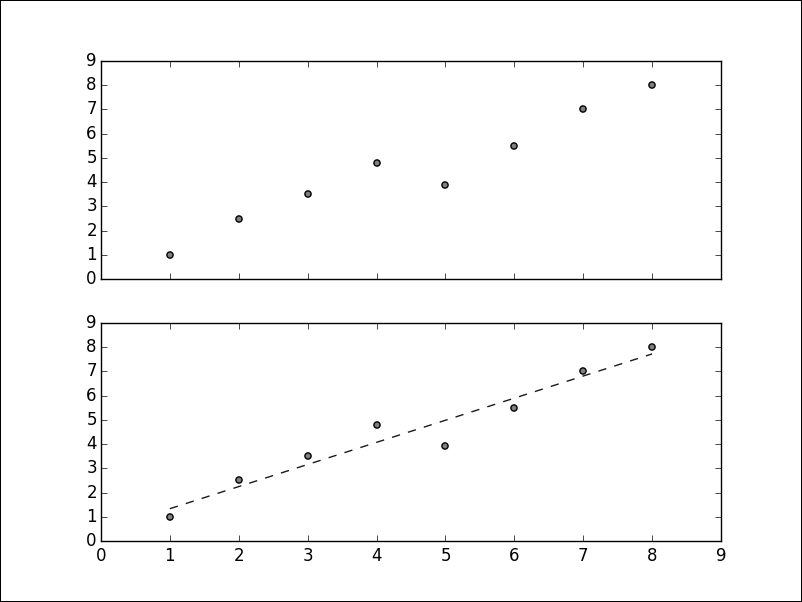
The above graph is a simple example with artificial data, but linear regression has a wide range of applications. If given the characteristics of real estate objects, we can learn to predict prices. If given the features of the galaxies, such as size, color, or brightness, it is possible to predict their distance. If given the data about household income and education level of parents, we can say something about the grades of their children.

There are numerous applications of linear regression everywhere, where one or more independent variables might be connected to one or more dependent variables.

A lot of existing data is not labeled. It is still possible to learn from data without labels with unsupervised models. A typical task during exploratory data analysis is to find related items or clusters. We can imagine the Iris dataset, but without the labels:

While the task seems much harder without labels, one group of measurements (in the lower-left) seems to stand apart. The goal of clustering algorithms is to identify these groups.

We will use K-Means clustering on the Iris dataset (without the labels). This algorithm expects the number of clusters to be specified in advance, which can be a disadvantage. K-Means will try to partition the dataset into groups, by minimizing the within-cluster sum of squares.

For example, we instantiate the KMeans model with n_clusters equal to 3:

>>> from sklearn.cluster import KMeans
>>> km = KMeans(n_clusters=3)

Similar to supervised algorithms, we can use the fit methods to train the model, but we only pass the data and not target labels:

>>> km.fit(iris.data)
KMeans(copy_x=True, init='k-means++', max_iter=300, n_clusters=3, n_init=10, n_jobs=1, precompute_distances='auto', random_state=None, tol=0.0001, verbose=0)

We already saw attributes ending with an underscore. In this case, the algorithm assigned a label to the training data, which can be inspected with the labels_ attribute:

>>> km.labels_
array([1, 1, 1, 1, 1, 1, ..., 0, 2, 0, 0, 2], dtype=int32)

We can already compare the result of these algorithms with our known target labels:

>>> iris.target
array([0, 0, 0, 0, 0, 0, ..., 2, 2, 2, 2, 2])

We quickly relabel the result to simplify the prediction error calculation:

>>> tr = {1: 0, 2: 1, 0: 2}
>>> predicted_labels = np.array([tr[i] for i in km.labels_])
>>> sum([p == t for (p, t) in zip(predicted_labels, iris.target)])
134

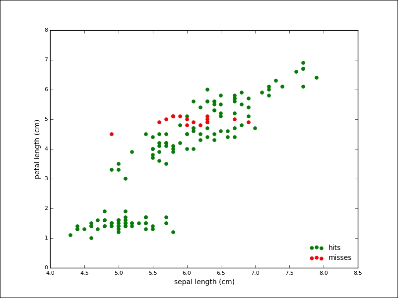
From 150 samples, K-Mean assigned the correct label to 134 samples, which is an accuracy of about 90 percent. The following plot shows the points of the algorithm predicted correctly in grey and the mislabeled points in red:

As another example for an unsupervised algorithm, we will take a look at Principal Component Analysis (PCA). The PCA aims to find the directions of the maximum variance in high-dimensional data. One goal is to reduce the number of dimensions by projecting a higher-dimensional space onto a lower-dimensional subspace while keeping most of the information.

The problem appears in various fields. You have collected many samples and each sample consists of hundreds or thousands of features. Not all the properties of the phenomenon at hand will be equally important. In our Iris dataset, we saw that the petal length alone seemed to be a good discriminator of the various species. PCA aims to find principal components that explain most of the variation in the data. If we sort our components accordingly (technically, we sort the eigenvectors of the covariance matrix by eigenvalue), we can keep the ones that explain most of the data and ignore the remaining ones, thereby reducing the dimensionality of the data.

It is simple to run PCA with scikit-learn. We will not go into the implementation details, but instead try to give you an intuition of PCA by running it on the Iris dataset, in order to give you yet another angle.

The process is similar to the ones we implemented so far. First, we instantiate our model; this time, the PCA from the decomposition submodule. We also import a standardization method, called StandardScaler, that will remove the mean from our data and scale to the unit variance. This step is a common requirement for many machine learning algorithms:

>>> from sklearn.decomposition import PCA
>>> from sklearn.preprocessing import StandardScaler

First, we instantiate our model with a parameter (which specifies the number of dimensions to reduce to), standardize our input, and run the fit_transform function that will take care of the mechanics of PCA:

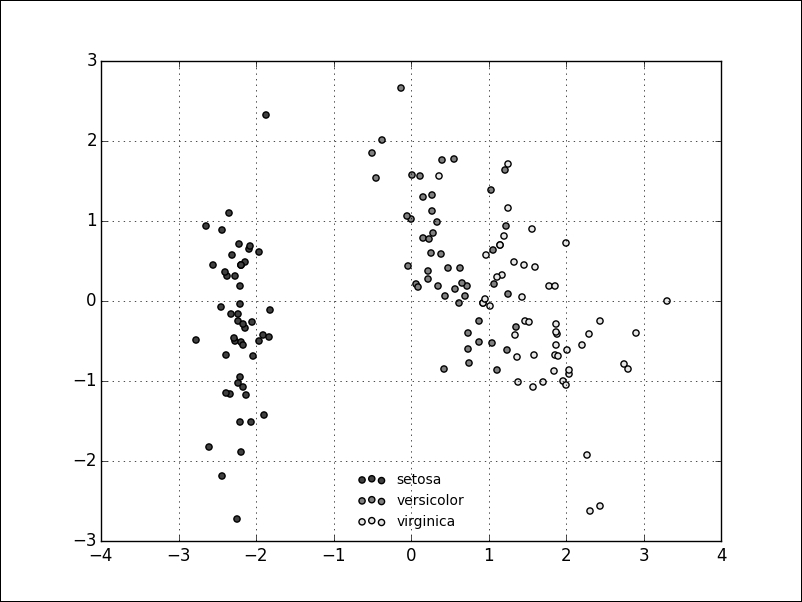
>>> pca = PCA(n_components=2)
>>> X = StandardScaler().fit_transform(iris.data)
>>> Y = pca.fit_transform(X)

The result is a dimensionality reduction in the Iris dataset from four (sepal and petal width and length) to two dimensions. It is important to note that this projection is not onto the two existing dimensions, so our new dataset does not consist of, for example, only petal length and width. Instead, the two new dimensions will represent a mixture of the existing features.

The following scatter plot shows the transformed dataset; from a glance at the plot, it looks like we still kept the essence of our dataset, even though we halved the number of dimensions:

Dimensionality reduction is just one way to deal with high-dimensional datasets, which are sometimes effected by the so called curse of dimensionality.

We have already seen that the machine learning process consists of the following steps:

So far, we omitted an important step that takes place between the training and application: the model testing and validation. In this step, we want to evaluate how well our model has learned.

One goal of learning, and machine learning in particular, is generalization. The question of whether a limited set of observations is enough to make statements about any possible observation is a deeper theoretical question, which is answered in dedicated resources on machine learning.

Whether or not a model generalizes well can also be tested. However, it is important that the training and the test input are separate. The situation where a model performs well on a training input but fails on an unseen test input is called overfitting, and this is not uncommon.

The basic approach is to split the available data into a training and test set, and scikit-learn helps to create this split with the train_test_split function.

We go back to the Iris dataset and perform SVC again. This time we will evaluate the performance of the algorithm on a training set. We set aside 40 percent of the data for testing:

>>> from sklearn.cross_validation import train_test_split
>>> X_train, X_test, y_train, y_test = train_test_split(iris.data, iris.target, test_size=0.4, random_state=0)
>>> clf = SVC()
>>> clf.fit(X_train, y_train)

The score function returns the mean accuracy of the given data and labels. We pass the test set for evaluation:

>>> clf.score(X_test, y_test)
 0.94999999999999996

The model seems to perform well, with about 94 percent accuracy on unseen data. We can now start to tweak model parameters (also called hyper parameters) to increase prediction performance. This cycle would bring back the problem of overfitting. One solution is to split the input data into three sets: one for training, validation, and testing. The iterative model of hyper-parameters tuning would take place between the training and the validation set, while the final evaluation would be done on the test set. Splitting the dataset into three reduces the number of samples we can learn from as well.

Cross-validation (CV) is a technique that does not need a validation set, but still counteracts overfitting. The dataset is split into k parts (called folds). For each fold, the model is trained on k-1 folds and tested on the remaining folds. The accuracy is taken as the average over the folds.

We will show a five-fold cross-validation on the Iris dataset, using SVC again:

>>> from sklearn.cross_validation import cross_val_score
>>> clf = SVC()
>>> scores = cross_val_score(clf, iris.data, iris.target, cv=5)
>>> scores
array([ 0.96666667,  1.    ,  0.96666667,  0.96666667,  1.    ])
>>> scores.mean()
0.98000000000000009

There are various strategies implemented by different classes to split the dataset for cross-validation: KFold, StratifiedKFold, LeaveOneOut, LeavePOut, LeaveOneLabelOut, LeavePLableOut, ShuffleSplit, StratifiedShuffleSplit, and PredefinedSplit.

Model verification is an important step and it is necessary for the development of robust machine learning solutions.

In this chapter, we took a whirlwind tour through one of the most popular Python machine learning libraries: scikit-learn. We saw what kind of data this library expects. Real-world data will seldom be ready to be fed into an estimator right away. With powerful libraries, such as Numpy and, especially, Pandas, you already saw how data can be retrieved, combined, and brought into shape. Visualization libraries, such as matplotlib, help along the way to get an intuition of the datasets, problems, and solutions.

During this chapter, we looked at a canonical dataset, the Iris dataset. We also looked at it from various angles: as a problem in supervised and unsupervised learning and as an example for model verification.

In total, we have looked at four different algorithms: the Support Vector Machine, Linear Regression, K-Means clustering, and Principal Component Analysis. Each of these alone is worth exploring, and we barely scratched the surface, although we were able to implement all the algorithms with only a few lines of Python.

There are numerous ways in which you can take your knowledge of the data analysis process further. Hundreds of books have been published on machine learning, so we only want to highlight a few here: Building Machine Learning Systems with Python by Richert and Coelho, will go much deeper into scikit-learn as we couldn't in this chapter. Learning from Data by Abu-Mostafa, Magdon-Ismail, and Lin, is a great resource for a solid theoretical foundation of learning problems in general.

The most interesting applications will be found in your own field. However, if you would like to get some inspiration, we recommend that you look at the www.kaggle.com website that runs predictive modeling and analytics competitions, which are both fun and insightful.

Practice exercises

Are the following problems supervised or unsupervised? Regression or classification problems?:

Look up one of the first machine learning models and algorithms: the perceptron. Try the perceptron on the Iris dataset and estimate the accuracy of the model. How does the perceptron compare to the SVC from this chapter?