

In this chapter, we will discuss the use of Wireshark for its primary purpose—troubleshooting network and application connectivity, functionality, and performance issues.
The topics that will be covered include:
- Troubleshooting methodology
- Troubleshooting connectivity issues
- Troubleshooting functional issues
- Performance analysis methodology
- Top five reasons for poor application performance
- Detecting and prioritizing delays
- Server processing time events
- Application turn's delay
- Network path latency
- Bandwidth congestion
- Data transport issues
These topics cover the majority of problems you'll come across in your analysis efforts.
There are two fundamental reasons why you might be doing packet analysis:
A third gray area is an application that basically works but is slow and occasionally times out, which could involve an underlying functional problem that causes the performance issue, or just simply be a really poor performance.
Troubleshooting a connectivity or functional issue is just a matter of comparing what normally works with what is going on, in the case you're working on.
A performance problem, on the other hand, requires determining where the majority of the time for a particular transaction to complete is being spent, measuring the delay and comparing that delay to what is normal or acceptable. The source and type of excessive delay usually points to the next area to investigate further or resolve.
In any case, you need to gather the information that allows you to determine whether this is a connectivity, functional, or performance issue and approach the problem according to its nature.
The most important thing you can do when approaching a problem is to determine what the real problem is so you can work on the right problem or the right aspect of the problem. In order to determine what the real problem is, or at least get close, you'll need to ask questions and interpret the answers. These questions could include the appropriate selections (depending on the complaint) from the following list:
- Define the problem:
- What were you trying to do (connect to a server, log in, send/receive e-mails, general application usage, upload/download file, and specific transactions or functions)?
- Is nothing working or is this just a problem with a specific application or multiple applications?
- What website/server/application were you trying / connecting to? Do you know the hostname, URL, and/or IP address and port used to access the application?
- What is the symptom/nature of the problem? Has this application or function/feature worked before, or is this the first time you've ever tried to use it?
- Did you receive any error messages or other indications of a problem?
- Is the issue consistent or intermittent? Depends? On what?
- How long has this been happening?
- Was there some recent change that did or could have had an impact?
- What has been identified or suspected so far? What has been done to address this? Has it helped or changed anything?
- Are there any other pertinent factors, symptoms, or recent changes to the user environment that should be considered?
- Determine the scope of the issue:
- Is this problem occurring for a single user or a group of users?
- Is this problem occurring within a specific office, region, or across the whole company?
- Is this problem affecting different types of users differently?
- Collect system, application, and path information. For a more in-depth analysis (beyond single user or small group issues), the applicable questions from the following list might also need to be gathered and analyzed, as appropriate to the complaint (some of this information may have to be obtained from network or application support groups):
- What is the browser type and version on the client (for web apps)? Is this different from clients that are working properly?
- What is the operating system type and version of the client(s) and server?
- What is the proper (vendor) application name and version? Are there any known issues with the application that match these symptoms (check the vendor's bug reports).
- What is the database type and server environment behind the application server?
- Are there other backend-supporting data sources such as an online data service or Documentum and SharePoint servers involved?
- What is the network path between the client and server? Are there firewalls, proxy servers, load balancers, and/or WAN accelerators in the path? Are they configured and working properly?
- Can you confirm the expected network path (and any WAN links involved) with a traceroute and verify the bandwidth availability?
- Can you measure the round trip time (RTT) path latency from the user to the application server with pings or TCP handshake completion times?
At this point, you should be able to identify the general nature of the problem between one of the following three basic types:
- Determine whether this is a connectivity problem
- User(s) cannot connect to anything
- User(s) cannot connect to a specific server/application
- Determine whether this is a functionality or configuration problem
- User(s) can connect (gets a login screen or other response from the application server) but cannot log in (or get the expected response)
- User(s) can connect and log in but some or all functions are failing (for example, cannot send/receive e-mails)
- Determine whether this is a performance problem
When I was doing component-level repair of electronic equipment early in my career, I learned to use the "half-split" troubleshooting method, which worked very well in almost every single case. Half-split troubleshooting is the process of cutting the problem domain (in my case, a piece of radio gear) in half by injecting or measuring signals roughly midway through the system. The idea is to see which half is working right and which half isn't, then shifting focus to the half that doesn't work, analyzing it halfway through, and so on. This process is repeated until you narrow the problem down to its source.
In the network and application world, the same half-split troubleshooting approach can be applied as well, in a general sense. If users are complaining that the network is slow, try to confirm or eliminate the network:
- Are users close to the server experiencing similar slowness? How about users in other remote locations?
- If a certain application is slow for a remote user, are other applications slow for that user as well?
- If users can't connect to a given server, can they connect to other servers nearby or at other locations?
By a process of logical examination of what does and doesn't work, you can eliminate a lot of guesswork and narrow your analysis down to just a few plausible possibilities.
It's usually much easier to determine the source of a connectivity or functionality problem if you have an environment where everything is working properly to compare with a situation that does not work. A packet capture of a working versus a non-working scenario can be compared to see what is different and if those differences are significant.
It is important not to make too many assumptions about a problem, even if the issue you're working on looks the same as the one that you've fixed before. Always verify the problem and the resolution that you should be able to apply and remove a fix and see the problem disappear/reappear reliably. Otherwise, you should question yourself about whether you've found the true source of the issue or are just affecting the symptoms.
Unless a reported problem is obviously a system-wide or specific server issue, it is better to conduct at least the initial analysis at or as close to the complaining user's workstation as possible. This has the advantages of offering the ability to perform the following actions:
- View and verify the actual problem that the user is reporting
- Measure round-trip times to the target server(s)
- Capture and view the TCP handshake process upon session initiation
- Capture and investigate the login and any other background processes and traffic
- Look for indications of network problems (lost packets and retransmissions) as they are experienced by the user's device
- Measure the apparent network throughput to the user's workstation during data downloads
- Eliminate the need to use a capture filter; the amount of traffic to/from a single workstation should not be excessive
A capture at a user workstation, server, or other device should be conducted with the use of an aggregating Test Access Point (TAP) versus using a switch SPAN port (as discussed in Chapter 3, Capturing All the Right Packets, or as a last resort by installing Wireshark on the user's workstation or server (if authorized).
Single user or small group connectivity issues can be resolved by confirming that the networking functions required for a user workstation to access local and remote network resources are functioning properly. The basic requirements or items to confirm include:
- Enabling the correct network interface(s) (workstation configuration)
- Confirming layer 1 (physical) connectivity
- Obtaining an IP address, subnet mask, and default gateway for each interface (DHCP)
- Obtaining the MAC address of the default gateway or other local network services (ARP)
- Obtaining the IP address of a network service (DNS)
- Connecting to a network service (TCP handshake or UDP response)
We'll briefly discuss each of these in order; while the first two steps will not involve using Wireshark, they are a necessary part in a troubleshooting approach. If the connectivity issue is affecting a group of users or a whole office, the first step is probably not applicable.
While it may seem obvious that network interfaces need to be enabled, the assumption that they are automatically enabled (especially for the wireless connectivity) by default upon device boot up may be false.
On Windows, you can use the command-line utility ipconfig to view the status and basic configuration (IP address, subnet mask, and default gateway) of network interfaces; on Linux or MAC devices, the equivalent command is ifconfig or ip.
If a connectivity problem is isolated to a single user's workstation, the physical connections are suspected. There are a few items to check, and the troubleshooting steps that can be taken are as follows:
- If there is a problem with the Ethernet cable from the workstation to a wall jack, you need to swap the cable with a different one.
- If there is a problem with the cabling from the user's wall jack to the switch port, you need to temporarily plug the user's Ethernet cable into another (known good) wall jack.
- If there is a problem with the switch, switch port, or port configuration, you need to temporarily plug the user's port cable into another (known good) port. Be aware that some network security policies call to disable switch ports until they are needed or configuring the port to be associated with a single, specific MAC address. If so, a port may not work when you plug into it although there is nothing physically wrong with it.
Unless the workstation was manually configured, it will need to get its IP address, subnet mask, default gateway, and DNS server settings from a DHCP server. If this does not appear to be working properly (after checking the configuration using ipconfig (Windows) or ifconfig, (Linux or Mac OS X)), you need to perform a packet capture during the workstation initialization/boot-up process using a TAP or SPAN port and investigate the DHCP requests and responses.
There are eight DHCP message types (not to be confused with the two Bootstrap Protocol types, Boot Request and Boot Reply):
For a workstation that is booting up and was previously working on the network, you'll generally see the DHCP Request and Acknowledgment packets verifying that the workstation can still use a previously leased address. On an entirely cold start up, the first two DHCP packets will be DHCP Discover and DHCP Offer packets, followed by the Request and ACK packets.
In a DHCPv6 environment, the typical packet sequence is DHCPv6 Solicit, DHCPv6 Advertise, DHCPv6 Request, and DHCPv6 Reply.
The fields to verify in a DHCP Response packet (or similar fields in a DHCPv6 Advertise packet) include the following four fields:
- Your (client) IP Address: This is the offered IP address for this workstation
- Subnet Mask: This is the subnet mask to use on this network
- Domain Name Server: This is the DNS server IP address
- Router: This is the IP address of the default gateway to use
This is minimum data required for any network communications; an example of these fields being provided in a DHCP Reply packet is illustrated in the following screenshot:

You can apply Wireshark display filters to isolate DHCP packets; the filter is bootp, as this is the legacy name for DHCP:
- DHCP display filter:
bootp bootp.option.dhcp == 5 (DHCP Message Type 'ACK') - DHCPv6 display filter:
dhcpv6 dhcpv6.msgtype == 2 (DHCPv6 'Advertise')
You can save the basic bootp and dhcpv6 display filters as a Filter Expression Button (FEB) after entering the filter string in the textbox on the Display Filter toolbar, clicking on Save, and giving the button a name such as DHCP Pkts and DHCPv6 Pkts respectively. Alternatively, you could combine both filters with an or (||) in one button, as shown in the following screenshot:

You might want to save another FEB that displays an abnormal DHCP condition packets using the following display filter string and call the DHCP Errors button or a similar as follows:
bootp.option.dhcp == 4 || bootp.option.dhcp == 6 || bootp.option.dhcp == 7
Similar abnormal event display filters for DHCPv6 could include:
dhcpv6.msgtype == 8 || dhcpv6.msgtype == 9 || dhcpv6.msgtype == 10
You can research more about DHCP, DHCPv6, and the various DHCPv6 message types online or from other sources if you need to analyze these in more detail.
A workstation will utilize the ARP protocol to obtain a MAC address for known IP addresses of network services, such as its default gateway or the DNS server if it's located on the same network segment. The ARP protocol and how it typically functions has already been covered in Chapter 2, Networking for Packet Analysts.
You may want to create an ARP FEB using the arp display filter syntax to make it quick and easy to inspect those packets.
A client workstation sends queries to a DNS server to obtain an IP address for a given hostname; the DNS server responds with the information or asks other DNS servers for the information on behalf of the client.
The format of the DNS query and response packet fields as displayed in the Wireshark Packet Details pane is fairly intuitive. An example of a DNS response packet containing a resolved IP address for time.windows.com, which actually provided the IP address (137.170.185.211) for the alias time.microsoft.akadns.com is shown in the following screenshot:

If a client workstation cannot obtain the IP address of a web service or application server, a packet-level investigation of the request (which URL or hostname is being requested), and what the response is from the DNS server (if any) should be revealing. A comparison of a failing query with queries that work properly for other hostnames or from other workstations should reveal the root of the problem (if DNS is the problem). Failure to obtain an IP address can be caused by an inoperable DNS server, improper hostname or URL, or a problem with connectivity from the user to other parts of the network, which we'll check next.
A few simple tests can confirm that basic network connectivity is working, or reveal a routing issue or another issue that needs to be addressed by the network support team.
Capturing and analyzing the ICMP packets sent and received during the following tests can be revealing; although, the test results themselves are often telling enough:
- Ping the user's default gateway using the default gateway IP address obtained from using
ipconfig /all(Windows) orip addr show(Linux) to confirm that the user workstation has basic connectivity on the local network. - Ping the hostname or URL of the target server. If this fails (request timed out message), try to ping other hosts or URLs. If necessary, inspect the DNS and/or ICMP responses in a packet capture of these tests to determine the nature of the failure. Otherwise, take note of the average round trip times.
- If a ping works to the default gateway but pinging other targets fails, a traceroute to a target server can reveal where in the network path connectivity ceases to function or is blocked.
Note
The traceroute command-line utility in Windows is
tracert, whereas for traceroutes on Linux/Unix and Mac OS X machines, the command istraceroute. To do a traceroute in Windows, open a Command Prompt (CMD) window and typetracert <hostname or IP Address of target>. In most other environments, open a terminal window and typetraceroute <hostname or IP address of target>.
If you can ping the target server and network connectivity is functioning, you can move on to the next step in the troubleshooting process. If not, be aware that some hosts may be configured to not respond to ICMP ping requests, and/or ICMP is blocked by a firewall between the user and server for security reasons. So, the inability to ping a device is not necessarily a sign of a network problem. Traceroute results should help determine how far and to what extent network connectivity is functioning in the path towards the target server; testing to other targets should be revealing as well.
An example of pinging a default gateway, then a URL, and finally performing a traceroute to the target URL is depicted in the following screenshot:
If network connectivity from a user workstation to a target server is functional (as proven by the ability to ping the host), a problem connecting to a specific application hosted on that server may be caused by a number of factors:
- The URL or port used by the client to access the application is wrong
- The port used to access the application is blocked by a firewall
- The application service is not turned up or is not working properly
The first of these factors is far more likely for a single user issue. Any of the last two factors would prevent anyone in a group or the whole organization from accessing the application. A packet-level analysis (from the client side) of a user attempting to connect to an application that is blocked should result in ICMP messages: Destination Host is Unreachable or Destination Port is Unreachable, or there will be no response at all if ICMP messages are being blocked by a firewall.
If the server is up, the application is reportedly operational but cannot be accessed; a client-side capture does not offer any solid clues, but a packet capture of the TCP session setup (if any) from or near the server end should be revealing.
Enabling network interfaces
While it may seem obvious that network interfaces need to be enabled, the assumption that they are automatically enabled (especially for the wireless connectivity) by default upon device boot up may be false.
On Windows, you can use the command-line utility ipconfig to view the status and basic configuration (IP address, subnet mask, and default gateway) of network interfaces; on Linux or MAC devices, the equivalent command is ifconfig or ip.
If a connectivity problem is isolated to a single user's workstation, the physical connections are suspected. There are a few items to check, and the troubleshooting steps that can be taken are as follows:
- If there is a problem with the Ethernet cable from the workstation to a wall jack, you need to swap the cable with a different one.
- If there is a problem with the cabling from the user's wall jack to the switch port, you need to temporarily plug the user's Ethernet cable into another (known good) wall jack.
- If there is a problem with the switch, switch port, or port configuration, you need to temporarily plug the user's port cable into another (known good) port. Be aware that some network security policies call to disable switch ports until they are needed or configuring the port to be associated with a single, specific MAC address. If so, a port may not work when you plug into it although there is nothing physically wrong with it.
Unless the workstation was manually configured, it will need to get its IP address, subnet mask, default gateway, and DNS server settings from a DHCP server. If this does not appear to be working properly (after checking the configuration using ipconfig (Windows) or ifconfig, (Linux or Mac OS X)), you need to perform a packet capture during the workstation initialization/boot-up process using a TAP or SPAN port and investigate the DHCP requests and responses.
There are eight DHCP message types (not to be confused with the two Bootstrap Protocol types, Boot Request and Boot Reply):
For a workstation that is booting up and was previously working on the network, you'll generally see the DHCP Request and Acknowledgment packets verifying that the workstation can still use a previously leased address. On an entirely cold start up, the first two DHCP packets will be DHCP Discover and DHCP Offer packets, followed by the Request and ACK packets.
In a DHCPv6 environment, the typical packet sequence is DHCPv6 Solicit, DHCPv6 Advertise, DHCPv6 Request, and DHCPv6 Reply.
The fields to verify in a DHCP Response packet (or similar fields in a DHCPv6 Advertise packet) include the following four fields:
- Your (client) IP Address: This is the offered IP address for this workstation
- Subnet Mask: This is the subnet mask to use on this network
- Domain Name Server: This is the DNS server IP address
- Router: This is the IP address of the default gateway to use
This is minimum data required for any network communications; an example of these fields being provided in a DHCP Reply packet is illustrated in the following screenshot:
You can apply Wireshark display filters to isolate DHCP packets; the filter is bootp, as this is the legacy name for DHCP:
- DHCP display filter:
bootp bootp.option.dhcp == 5 (DHCP Message Type 'ACK') - DHCPv6 display filter:
dhcpv6 dhcpv6.msgtype == 2 (DHCPv6 'Advertise')
You can save the basic bootp and dhcpv6 display filters as a Filter Expression Button (FEB) after entering the filter string in the textbox on the Display Filter toolbar, clicking on Save, and giving the button a name such as DHCP Pkts and DHCPv6 Pkts respectively. Alternatively, you could combine both filters with an or (||) in one button, as shown in the following screenshot:
You might want to save another FEB that displays an abnormal DHCP condition packets using the following display filter string and call the DHCP Errors button or a similar as follows:
bootp.option.dhcp == 4 || bootp.option.dhcp == 6 || bootp.option.dhcp == 7
Similar abnormal event display filters for DHCPv6 could include:
dhcpv6.msgtype == 8 || dhcpv6.msgtype == 9 || dhcpv6.msgtype == 10
You can research more about DHCP, DHCPv6, and the various DHCPv6 message types online or from other sources if you need to analyze these in more detail.
A workstation will utilize the ARP protocol to obtain a MAC address for known IP addresses of network services, such as its default gateway or the DNS server if it's located on the same network segment. The ARP protocol and how it typically functions has already been covered in Chapter 2, Networking for Packet Analysts.
You may want to create an ARP FEB using the arp display filter syntax to make it quick and easy to inspect those packets.
A client workstation sends queries to a DNS server to obtain an IP address for a given hostname; the DNS server responds with the information or asks other DNS servers for the information on behalf of the client.
The format of the DNS query and response packet fields as displayed in the Wireshark Packet Details pane is fairly intuitive. An example of a DNS response packet containing a resolved IP address for time.windows.com, which actually provided the IP address (137.170.185.211) for the alias time.microsoft.akadns.com is shown in the following screenshot:
If a client workstation cannot obtain the IP address of a web service or application server, a packet-level investigation of the request (which URL or hostname is being requested), and what the response is from the DNS server (if any) should be revealing. A comparison of a failing query with queries that work properly for other hostnames or from other workstations should reveal the root of the problem (if DNS is the problem). Failure to obtain an IP address can be caused by an inoperable DNS server, improper hostname or URL, or a problem with connectivity from the user to other parts of the network, which we'll check next.
A few simple tests can confirm that basic network connectivity is working, or reveal a routing issue or another issue that needs to be addressed by the network support team.
Capturing and analyzing the ICMP packets sent and received during the following tests can be revealing; although, the test results themselves are often telling enough:
- Ping the user's default gateway using the default gateway IP address obtained from using
ipconfig /all(Windows) orip addr show(Linux) to confirm that the user workstation has basic connectivity on the local network. - Ping the hostname or URL of the target server. If this fails (request timed out message), try to ping other hosts or URLs. If necessary, inspect the DNS and/or ICMP responses in a packet capture of these tests to determine the nature of the failure. Otherwise, take note of the average round trip times.
- If a ping works to the default gateway but pinging other targets fails, a traceroute to a target server can reveal where in the network path connectivity ceases to function or is blocked.
Note
The traceroute command-line utility in Windows is
tracert, whereas for traceroutes on Linux/Unix and Mac OS X machines, the command istraceroute. To do a traceroute in Windows, open a Command Prompt (CMD) window and typetracert <hostname or IP Address of target>. In most other environments, open a terminal window and typetraceroute <hostname or IP address of target>.
If you can ping the target server and network connectivity is functioning, you can move on to the next step in the troubleshooting process. If not, be aware that some hosts may be configured to not respond to ICMP ping requests, and/or ICMP is blocked by a firewall between the user and server for security reasons. So, the inability to ping a device is not necessarily a sign of a network problem. Traceroute results should help determine how far and to what extent network connectivity is functioning in the path towards the target server; testing to other targets should be revealing as well.
An example of pinging a default gateway, then a URL, and finally performing a traceroute to the target URL is depicted in the following screenshot:
If network connectivity from a user workstation to a target server is functional (as proven by the ability to ping the host), a problem connecting to a specific application hosted on that server may be caused by a number of factors:
- The URL or port used by the client to access the application is wrong
- The port used to access the application is blocked by a firewall
- The application service is not turned up or is not working properly
The first of these factors is far more likely for a single user issue. Any of the last two factors would prevent anyone in a group or the whole organization from accessing the application. A packet-level analysis (from the client side) of a user attempting to connect to an application that is blocked should result in ICMP messages: Destination Host is Unreachable or Destination Port is Unreachable, or there will be no response at all if ICMP messages are being blocked by a firewall.
If the server is up, the application is reportedly operational but cannot be accessed; a client-side capture does not offer any solid clues, but a packet capture of the TCP session setup (if any) from or near the server end should be revealing.
Confirming physical connectivity
If a connectivity problem is isolated to a single user's workstation, the physical connections are suspected. There are a few items to check, and the troubleshooting steps that can be taken are as follows:
- If there is a problem with the Ethernet cable from the workstation to a wall jack, you need to swap the cable with a different one.
- If there is a problem with the cabling from the user's wall jack to the switch port, you need to temporarily plug the user's Ethernet cable into another (known good) wall jack.
- If there is a problem with the switch, switch port, or port configuration, you need to temporarily plug the user's port cable into another (known good) port. Be aware that some network security policies call to disable switch ports until they are needed or configuring the port to be associated with a single, specific MAC address. If so, a port may not work when you plug into it although there is nothing physically wrong with it.
Unless the workstation was manually configured, it will need to get its IP address, subnet mask, default gateway, and DNS server settings from a DHCP server. If this does not appear to be working properly (after checking the configuration using ipconfig (Windows) or ifconfig, (Linux or Mac OS X)), you need to perform a packet capture during the workstation initialization/boot-up process using a TAP or SPAN port and investigate the DHCP requests and responses.
There are eight DHCP message types (not to be confused with the two Bootstrap Protocol types, Boot Request and Boot Reply):
For a workstation that is booting up and was previously working on the network, you'll generally see the DHCP Request and Acknowledgment packets verifying that the workstation can still use a previously leased address. On an entirely cold start up, the first two DHCP packets will be DHCP Discover and DHCP Offer packets, followed by the Request and ACK packets.
In a DHCPv6 environment, the typical packet sequence is DHCPv6 Solicit, DHCPv6 Advertise, DHCPv6 Request, and DHCPv6 Reply.
The fields to verify in a DHCP Response packet (or similar fields in a DHCPv6 Advertise packet) include the following four fields:
- Your (client) IP Address: This is the offered IP address for this workstation
- Subnet Mask: This is the subnet mask to use on this network
- Domain Name Server: This is the DNS server IP address
- Router: This is the IP address of the default gateway to use
This is minimum data required for any network communications; an example of these fields being provided in a DHCP Reply packet is illustrated in the following screenshot:
You can apply Wireshark display filters to isolate DHCP packets; the filter is bootp, as this is the legacy name for DHCP:
- DHCP display filter:
bootp bootp.option.dhcp == 5 (DHCP Message Type 'ACK') - DHCPv6 display filter:
dhcpv6 dhcpv6.msgtype == 2 (DHCPv6 'Advertise')
You can save the basic bootp and dhcpv6 display filters as a Filter Expression Button (FEB) after entering the filter string in the textbox on the Display Filter toolbar, clicking on Save, and giving the button a name such as DHCP Pkts and DHCPv6 Pkts respectively. Alternatively, you could combine both filters with an or (||) in one button, as shown in the following screenshot:
You might want to save another FEB that displays an abnormal DHCP condition packets using the following display filter string and call the DHCP Errors button or a similar as follows:
bootp.option.dhcp == 4 || bootp.option.dhcp == 6 || bootp.option.dhcp == 7
Similar abnormal event display filters for DHCPv6 could include:
dhcpv6.msgtype == 8 || dhcpv6.msgtype == 9 || dhcpv6.msgtype == 10
You can research more about DHCP, DHCPv6, and the various DHCPv6 message types online or from other sources if you need to analyze these in more detail.
A workstation will utilize the ARP protocol to obtain a MAC address for known IP addresses of network services, such as its default gateway or the DNS server if it's located on the same network segment. The ARP protocol and how it typically functions has already been covered in Chapter 2, Networking for Packet Analysts.
You may want to create an ARP FEB using the arp display filter syntax to make it quick and easy to inspect those packets.
A client workstation sends queries to a DNS server to obtain an IP address for a given hostname; the DNS server responds with the information or asks other DNS servers for the information on behalf of the client.
The format of the DNS query and response packet fields as displayed in the Wireshark Packet Details pane is fairly intuitive. An example of a DNS response packet containing a resolved IP address for time.windows.com, which actually provided the IP address (137.170.185.211) for the alias time.microsoft.akadns.com is shown in the following screenshot:
If a client workstation cannot obtain the IP address of a web service or application server, a packet-level investigation of the request (which URL or hostname is being requested), and what the response is from the DNS server (if any) should be revealing. A comparison of a failing query with queries that work properly for other hostnames or from other workstations should reveal the root of the problem (if DNS is the problem). Failure to obtain an IP address can be caused by an inoperable DNS server, improper hostname or URL, or a problem with connectivity from the user to other parts of the network, which we'll check next.
A few simple tests can confirm that basic network connectivity is working, or reveal a routing issue or another issue that needs to be addressed by the network support team.
Capturing and analyzing the ICMP packets sent and received during the following tests can be revealing; although, the test results themselves are often telling enough:
- Ping the user's default gateway using the default gateway IP address obtained from using
ipconfig /all(Windows) orip addr show(Linux) to confirm that the user workstation has basic connectivity on the local network. - Ping the hostname or URL of the target server. If this fails (request timed out message), try to ping other hosts or URLs. If necessary, inspect the DNS and/or ICMP responses in a packet capture of these tests to determine the nature of the failure. Otherwise, take note of the average round trip times.
- If a ping works to the default gateway but pinging other targets fails, a traceroute to a target server can reveal where in the network path connectivity ceases to function or is blocked.
Note
The traceroute command-line utility in Windows is
tracert, whereas for traceroutes on Linux/Unix and Mac OS X machines, the command istraceroute. To do a traceroute in Windows, open a Command Prompt (CMD) window and typetracert <hostname or IP Address of target>. In most other environments, open a terminal window and typetraceroute <hostname or IP address of target>.
If you can ping the target server and network connectivity is functioning, you can move on to the next step in the troubleshooting process. If not, be aware that some hosts may be configured to not respond to ICMP ping requests, and/or ICMP is blocked by a firewall between the user and server for security reasons. So, the inability to ping a device is not necessarily a sign of a network problem. Traceroute results should help determine how far and to what extent network connectivity is functioning in the path towards the target server; testing to other targets should be revealing as well.
An example of pinging a default gateway, then a URL, and finally performing a traceroute to the target URL is depicted in the following screenshot:
If network connectivity from a user workstation to a target server is functional (as proven by the ability to ping the host), a problem connecting to a specific application hosted on that server may be caused by a number of factors:
- The URL or port used by the client to access the application is wrong
- The port used to access the application is blocked by a firewall
- The application service is not turned up or is not working properly
The first of these factors is far more likely for a single user issue. Any of the last two factors would prevent anyone in a group or the whole organization from accessing the application. A packet-level analysis (from the client side) of a user attempting to connect to an application that is blocked should result in ICMP messages: Destination Host is Unreachable or Destination Port is Unreachable, or there will be no response at all if ICMP messages are being blocked by a firewall.
If the server is up, the application is reportedly operational but cannot be accessed; a client-side capture does not offer any solid clues, but a packet capture of the TCP session setup (if any) from or near the server end should be revealing.
Obtaining the workstation IP configuration
Unless the workstation was manually configured, it will need to get its IP address, subnet mask, default gateway, and DNS server settings from a DHCP server. If this does not appear to be working properly (after checking the configuration using ipconfig (Windows) or ifconfig, (Linux or Mac OS X)), you need to perform a packet capture during the workstation initialization/boot-up process using a TAP or SPAN port and investigate the DHCP requests and responses.
There are eight DHCP message types (not to be confused with the two Bootstrap Protocol types, Boot Request and Boot Reply):
For a workstation that is booting up and was previously working on the network, you'll generally see the DHCP Request and Acknowledgment packets verifying that the workstation can still use a previously leased address. On an entirely cold start up, the first two DHCP packets will be DHCP Discover and DHCP Offer packets, followed by the Request and ACK packets.
In a DHCPv6 environment, the typical packet sequence is DHCPv6 Solicit, DHCPv6 Advertise, DHCPv6 Request, and DHCPv6 Reply.
The fields to verify in a DHCP Response packet (or similar fields in a DHCPv6 Advertise packet) include the following four fields:
- Your (client) IP Address: This is the offered IP address for this workstation
- Subnet Mask: This is the subnet mask to use on this network
- Domain Name Server: This is the DNS server IP address
- Router: This is the IP address of the default gateway to use
This is minimum data required for any network communications; an example of these fields being provided in a DHCP Reply packet is illustrated in the following screenshot:
You can apply Wireshark display filters to isolate DHCP packets; the filter is bootp, as this is the legacy name for DHCP:
- DHCP display filter:
bootp bootp.option.dhcp == 5 (DHCP Message Type 'ACK') - DHCPv6 display filter:
dhcpv6 dhcpv6.msgtype == 2 (DHCPv6 'Advertise')
You can save the basic bootp and dhcpv6 display filters as a Filter Expression Button (FEB) after entering the filter string in the textbox on the Display Filter toolbar, clicking on Save, and giving the button a name such as DHCP Pkts and DHCPv6 Pkts respectively. Alternatively, you could combine both filters with an or (||) in one button, as shown in the following screenshot:
You might want to save another FEB that displays an abnormal DHCP condition packets using the following display filter string and call the DHCP Errors button or a similar as follows:
bootp.option.dhcp == 4 || bootp.option.dhcp == 6 || bootp.option.dhcp == 7
Similar abnormal event display filters for DHCPv6 could include:
dhcpv6.msgtype == 8 || dhcpv6.msgtype == 9 || dhcpv6.msgtype == 10
You can research more about DHCP, DHCPv6, and the various DHCPv6 message types online or from other sources if you need to analyze these in more detail.
A workstation will utilize the ARP protocol to obtain a MAC address for known IP addresses of network services, such as its default gateway or the DNS server if it's located on the same network segment. The ARP protocol and how it typically functions has already been covered in Chapter 2, Networking for Packet Analysts.
You may want to create an ARP FEB using the arp display filter syntax to make it quick and easy to inspect those packets.
A client workstation sends queries to a DNS server to obtain an IP address for a given hostname; the DNS server responds with the information or asks other DNS servers for the information on behalf of the client.
The format of the DNS query and response packet fields as displayed in the Wireshark Packet Details pane is fairly intuitive. An example of a DNS response packet containing a resolved IP address for time.windows.com, which actually provided the IP address (137.170.185.211) for the alias time.microsoft.akadns.com is shown in the following screenshot:
If a client workstation cannot obtain the IP address of a web service or application server, a packet-level investigation of the request (which URL or hostname is being requested), and what the response is from the DNS server (if any) should be revealing. A comparison of a failing query with queries that work properly for other hostnames or from other workstations should reveal the root of the problem (if DNS is the problem). Failure to obtain an IP address can be caused by an inoperable DNS server, improper hostname or URL, or a problem with connectivity from the user to other parts of the network, which we'll check next.
A few simple tests can confirm that basic network connectivity is working, or reveal a routing issue or another issue that needs to be addressed by the network support team.
Capturing and analyzing the ICMP packets sent and received during the following tests can be revealing; although, the test results themselves are often telling enough:
- Ping the user's default gateway using the default gateway IP address obtained from using
ipconfig /all(Windows) orip addr show(Linux) to confirm that the user workstation has basic connectivity on the local network. - Ping the hostname or URL of the target server. If this fails (request timed out message), try to ping other hosts or URLs. If necessary, inspect the DNS and/or ICMP responses in a packet capture of these tests to determine the nature of the failure. Otherwise, take note of the average round trip times.
- If a ping works to the default gateway but pinging other targets fails, a traceroute to a target server can reveal where in the network path connectivity ceases to function or is blocked.
Note
The traceroute command-line utility in Windows is
tracert, whereas for traceroutes on Linux/Unix and Mac OS X machines, the command istraceroute. To do a traceroute in Windows, open a Command Prompt (CMD) window and typetracert <hostname or IP Address of target>. In most other environments, open a terminal window and typetraceroute <hostname or IP address of target>.
If you can ping the target server and network connectivity is functioning, you can move on to the next step in the troubleshooting process. If not, be aware that some hosts may be configured to not respond to ICMP ping requests, and/or ICMP is blocked by a firewall between the user and server for security reasons. So, the inability to ping a device is not necessarily a sign of a network problem. Traceroute results should help determine how far and to what extent network connectivity is functioning in the path towards the target server; testing to other targets should be revealing as well.
An example of pinging a default gateway, then a URL, and finally performing a traceroute to the target URL is depicted in the following screenshot:
If network connectivity from a user workstation to a target server is functional (as proven by the ability to ping the host), a problem connecting to a specific application hosted on that server may be caused by a number of factors:
- The URL or port used by the client to access the application is wrong
- The port used to access the application is blocked by a firewall
- The application service is not turned up or is not working properly
The first of these factors is far more likely for a single user issue. Any of the last two factors would prevent anyone in a group or the whole organization from accessing the application. A packet-level analysis (from the client side) of a user attempting to connect to an application that is blocked should result in ICMP messages: Destination Host is Unreachable or Destination Port is Unreachable, or there will be no response at all if ICMP messages are being blocked by a firewall.
If the server is up, the application is reportedly operational but cannot be accessed; a client-side capture does not offer any solid clues, but a packet capture of the TCP session setup (if any) from or near the server end should be revealing.
Obtaining MAC addresses
A workstation will utilize the ARP protocol to obtain a MAC address for known IP addresses of network services, such as its default gateway or the DNS server if it's located on the same network segment. The ARP protocol and how it typically functions has already been covered in Chapter 2, Networking for Packet Analysts.
You may want to create an ARP FEB using the arp display filter syntax to make it quick and easy to inspect those packets.
A client workstation sends queries to a DNS server to obtain an IP address for a given hostname; the DNS server responds with the information or asks other DNS servers for the information on behalf of the client.
The format of the DNS query and response packet fields as displayed in the Wireshark Packet Details pane is fairly intuitive. An example of a DNS response packet containing a resolved IP address for time.windows.com, which actually provided the IP address (137.170.185.211) for the alias time.microsoft.akadns.com is shown in the following screenshot:
If a client workstation cannot obtain the IP address of a web service or application server, a packet-level investigation of the request (which URL or hostname is being requested), and what the response is from the DNS server (if any) should be revealing. A comparison of a failing query with queries that work properly for other hostnames or from other workstations should reveal the root of the problem (if DNS is the problem). Failure to obtain an IP address can be caused by an inoperable DNS server, improper hostname or URL, or a problem with connectivity from the user to other parts of the network, which we'll check next.
A few simple tests can confirm that basic network connectivity is working, or reveal a routing issue or another issue that needs to be addressed by the network support team.
Capturing and analyzing the ICMP packets sent and received during the following tests can be revealing; although, the test results themselves are often telling enough:
- Ping the user's default gateway using the default gateway IP address obtained from using
ipconfig /all(Windows) orip addr show(Linux) to confirm that the user workstation has basic connectivity on the local network. - Ping the hostname or URL of the target server. If this fails (request timed out message), try to ping other hosts or URLs. If necessary, inspect the DNS and/or ICMP responses in a packet capture of these tests to determine the nature of the failure. Otherwise, take note of the average round trip times.
- If a ping works to the default gateway but pinging other targets fails, a traceroute to a target server can reveal where in the network path connectivity ceases to function or is blocked.
Note
The traceroute command-line utility in Windows is
tracert, whereas for traceroutes on Linux/Unix and Mac OS X machines, the command istraceroute. To do a traceroute in Windows, open a Command Prompt (CMD) window and typetracert <hostname or IP Address of target>. In most other environments, open a terminal window and typetraceroute <hostname or IP address of target>.
If you can ping the target server and network connectivity is functioning, you can move on to the next step in the troubleshooting process. If not, be aware that some hosts may be configured to not respond to ICMP ping requests, and/or ICMP is blocked by a firewall between the user and server for security reasons. So, the inability to ping a device is not necessarily a sign of a network problem. Traceroute results should help determine how far and to what extent network connectivity is functioning in the path towards the target server; testing to other targets should be revealing as well.
An example of pinging a default gateway, then a URL, and finally performing a traceroute to the target URL is depicted in the following screenshot:
If network connectivity from a user workstation to a target server is functional (as proven by the ability to ping the host), a problem connecting to a specific application hosted on that server may be caused by a number of factors:
- The URL or port used by the client to access the application is wrong
- The port used to access the application is blocked by a firewall
- The application service is not turned up or is not working properly
The first of these factors is far more likely for a single user issue. Any of the last two factors would prevent anyone in a group or the whole organization from accessing the application. A packet-level analysis (from the client side) of a user attempting to connect to an application that is blocked should result in ICMP messages: Destination Host is Unreachable or Destination Port is Unreachable, or there will be no response at all if ICMP messages are being blocked by a firewall.
If the server is up, the application is reportedly operational but cannot be accessed; a client-side capture does not offer any solid clues, but a packet capture of the TCP session setup (if any) from or near the server end should be revealing.
Obtaining network service IP addresses
A client workstation sends queries to a DNS server to obtain an IP address for a given hostname; the DNS server responds with the information or asks other DNS servers for the information on behalf of the client.
The format of the DNS query and response packet fields as displayed in the Wireshark Packet Details pane is fairly intuitive. An example of a DNS response packet containing a resolved IP address for time.windows.com, which actually provided the IP address (137.170.185.211) for the alias time.microsoft.akadns.com is shown in the following screenshot:
If a client workstation cannot obtain the IP address of a web service or application server, a packet-level investigation of the request (which URL or hostname is being requested), and what the response is from the DNS server (if any) should be revealing. A comparison of a failing query with queries that work properly for other hostnames or from other workstations should reveal the root of the problem (if DNS is the problem). Failure to obtain an IP address can be caused by an inoperable DNS server, improper hostname or URL, or a problem with connectivity from the user to other parts of the network, which we'll check next.
A few simple tests can confirm that basic network connectivity is working, or reveal a routing issue or another issue that needs to be addressed by the network support team.
Capturing and analyzing the ICMP packets sent and received during the following tests can be revealing; although, the test results themselves are often telling enough:
- Ping the user's default gateway using the default gateway IP address obtained from using
ipconfig /all(Windows) orip addr show(Linux) to confirm that the user workstation has basic connectivity on the local network. - Ping the hostname or URL of the target server. If this fails (request timed out message), try to ping other hosts or URLs. If necessary, inspect the DNS and/or ICMP responses in a packet capture of these tests to determine the nature of the failure. Otherwise, take note of the average round trip times.
- If a ping works to the default gateway but pinging other targets fails, a traceroute to a target server can reveal where in the network path connectivity ceases to function or is blocked.
Note
The traceroute command-line utility in Windows is
tracert, whereas for traceroutes on Linux/Unix and Mac OS X machines, the command istraceroute. To do a traceroute in Windows, open a Command Prompt (CMD) window and typetracert <hostname or IP Address of target>. In most other environments, open a terminal window and typetraceroute <hostname or IP address of target>.
If you can ping the target server and network connectivity is functioning, you can move on to the next step in the troubleshooting process. If not, be aware that some hosts may be configured to not respond to ICMP ping requests, and/or ICMP is blocked by a firewall between the user and server for security reasons. So, the inability to ping a device is not necessarily a sign of a network problem. Traceroute results should help determine how far and to what extent network connectivity is functioning in the path towards the target server; testing to other targets should be revealing as well.
An example of pinging a default gateway, then a URL, and finally performing a traceroute to the target URL is depicted in the following screenshot:
If network connectivity from a user workstation to a target server is functional (as proven by the ability to ping the host), a problem connecting to a specific application hosted on that server may be caused by a number of factors:
- The URL or port used by the client to access the application is wrong
- The port used to access the application is blocked by a firewall
- The application service is not turned up or is not working properly
The first of these factors is far more likely for a single user issue. Any of the last two factors would prevent anyone in a group or the whole organization from accessing the application. A packet-level analysis (from the client side) of a user attempting to connect to an application that is blocked should result in ICMP messages: Destination Host is Unreachable or Destination Port is Unreachable, or there will be no response at all if ICMP messages are being blocked by a firewall.
If the server is up, the application is reportedly operational but cannot be accessed; a client-side capture does not offer any solid clues, but a packet capture of the TCP session setup (if any) from or near the server end should be revealing.
Basic network connectivity
A few simple tests can confirm that basic network connectivity is working, or reveal a routing issue or another issue that needs to be addressed by the network support team.
Capturing and analyzing the ICMP packets sent and received during the following tests can be revealing; although, the test results themselves are often telling enough:
- Ping the user's default gateway using the default gateway IP address obtained from using
ipconfig /all(Windows) orip addr show(Linux) to confirm that the user workstation has basic connectivity on the local network. - Ping the hostname or URL of the target server. If this fails (request timed out message), try to ping other hosts or URLs. If necessary, inspect the DNS and/or ICMP responses in a packet capture of these tests to determine the nature of the failure. Otherwise, take note of the average round trip times.
- If a ping works to the default gateway but pinging other targets fails, a traceroute to a target server can reveal where in the network path connectivity ceases to function or is blocked.
Note
The traceroute command-line utility in Windows is
tracert, whereas for traceroutes on Linux/Unix and Mac OS X machines, the command istraceroute. To do a traceroute in Windows, open a Command Prompt (CMD) window and typetracert <hostname or IP Address of target>. In most other environments, open a terminal window and typetraceroute <hostname or IP address of target>.
If you can ping the target server and network connectivity is functioning, you can move on to the next step in the troubleshooting process. If not, be aware that some hosts may be configured to not respond to ICMP ping requests, and/or ICMP is blocked by a firewall between the user and server for security reasons. So, the inability to ping a device is not necessarily a sign of a network problem. Traceroute results should help determine how far and to what extent network connectivity is functioning in the path towards the target server; testing to other targets should be revealing as well.
An example of pinging a default gateway, then a URL, and finally performing a traceroute to the target URL is depicted in the following screenshot:
If network connectivity from a user workstation to a target server is functional (as proven by the ability to ping the host), a problem connecting to a specific application hosted on that server may be caused by a number of factors:
- The URL or port used by the client to access the application is wrong
- The port used to access the application is blocked by a firewall
- The application service is not turned up or is not working properly
The first of these factors is far more likely for a single user issue. Any of the last two factors would prevent anyone in a group or the whole organization from accessing the application. A packet-level analysis (from the client side) of a user attempting to connect to an application that is blocked should result in ICMP messages: Destination Host is Unreachable or Destination Port is Unreachable, or there will be no response at all if ICMP messages are being blocked by a firewall.
If the server is up, the application is reportedly operational but cannot be accessed; a client-side capture does not offer any solid clues, but a packet capture of the TCP session setup (if any) from or near the server end should be revealing.
Connecting to the application services
If network connectivity from a user workstation to a target server is functional (as proven by the ability to ping the host), a problem connecting to a specific application hosted on that server may be caused by a number of factors:
- The URL or port used by the client to access the application is wrong
- The port used to access the application is blocked by a firewall
- The application service is not turned up or is not working properly
The first of these factors is far more likely for a single user issue. Any of the last two factors would prevent anyone in a group or the whole organization from accessing the application. A packet-level analysis (from the client side) of a user attempting to connect to an application that is blocked should result in ICMP messages: Destination Host is Unreachable or Destination Port is Unreachable, or there will be no response at all if ICMP messages are being blocked by a firewall.
If the server is up, the application is reportedly operational but cannot be accessed; a client-side capture does not offer any solid clues, but a packet capture of the TCP session setup (if any) from or near the server end should be revealing.
If a user is able to connect and set up a TCP session with an application server, but the application does not function otherwise, or function correctly, then, there are a number of areas that can be investigated. These areas can be investigated using a combination of packet-level analysis, error reports, and configuration comparisons with captures and configurations from other users' machines:
- User credentials: The most common reason for specific-user issues with application functionality is the lack of proper credentials, authorization, rights, and so on. This is the first thing to check whether other users are working normally.
- Application settings on the user machine: Some applications require specific configuration files to be placed on a user's machine in a specific location. Applications may also require certain version levels of application-specific utilities, Java, .NET frameworks, and so on. Usually, an application will provide an error message indicating at least the general nature of a configuration problem.
- Application reported errors: You can look for the error code within response packets or on the user screen that may reveal the nature of application errors:
- Differences in web browsers: Some web applications are designed to work with specific browsers (Chrome, Internet Explorer, Firefox, Opera, and so on) and may not work properly or at all on other browsers and there may not be any error messages provided that indicate this is the case. A comparison of the browser type and version with other working users may be revealing.
The causes of network connectivity and application functionality issues can vary widely, so it is impossible to draw a clear roadmap for every possibility. The best approach to successfully address these problems is not to make too many assumptions without proving those assumptions correct with systematic, logical troubleshooting steps, but try to find or create a scenario where the system, or at least part of the system, works properly and compare the appropriate packet-level details of the working environment to the one that doesn't work.
Analyzing an application's performance problem is basically a case of identifying where the majority of the time for a particular task to complete is being spent, and measuring/comparing that time to what is normal and/or acceptable for that type of task.
Generally speaking, performance issues can be attributed to one of the following five areas, in order of decreasing likelihood:
- Server processing time delay
- Application turns delay
- Network path latency
- Bandwidth congestion
- Data transport (TCP) issues
Client processing time is usually a relatively small component of overall response time—except perhaps for some compute-extensive desktop applications, which leaves the focus on the network and server environments and any performance-affecting application design characteristics.
As was done when preparing to troubleshoot a connectivity or functionality problem, you'll need to gather the right information about the application environment and problem domain. You'll also want to determine which tools you may need to use during the analysis: Wireshark, TAPs to facilitate packet captures, and any other analysis tools.
You will also need to determine where to perform the first packet capture:
- A client-side capture is the best place to begin a performance analysis effort. From this vantage point, you can view and verify what the user is complaining about, view any error messages presented to the user or evident in the packet capture, measure network round-trip times, and capture the performance characteristics to study within a packet capture without the need to use a capture filter so you know you won't miss anything.
- A server-side capture may be needed because a client-side capture may not be possible for a user that is at a long distance, or to analyze server-to-server transactions to backend databases or other data sources.
- A packet capture at some intermediate point in the network path may be needed to isolate the source of excessive packet loss/errors and the associated retransmissions.
Remember that the use of an aggregating TAP is preferable over using SPAN ports, or you can install Wireshark on the client workstation or server as a last resort, but get the capture done any way you have to.
After performing the capture and saving the bulk capture file, confirm the following:
- Check the file to ensure there are no packets with the ACKed Unseen Segment messages in the Wireshark Warnings tab in the Expert Info menu, which means Wireshark saw a packet that was acknowledged but didn't see the original packet; an indication that Wireshark is missing packets due to a bad TAP or SPAN port configuration or excessive traffic levels. In any case, if more than just a few of these show up, you'll want to do the capture again after confirming the capture setup.
- Next, you'll want to review the captured conversations in IPv4 in the Conversations window and sort the Bytes column. The IP conversation between the user and application server should be at or near the top so you can select this conversation, right-click on it, and select A <-> B in the Selected menu.
- After reviewing the filtered data to ensure it contains what you expected, select Export Specified Packets from the File menu and save the filtered capture file with a filename that reflects the fact that this is a filtered subset of the bulk capture file.
- Finally, open the filtered file you just saved so you're working with a smaller, faster file without any distracting packets from other conversations that have nothing to do with your analysis.
At the onset of your analysis, you should take a look through the Errors, Warnings, and Notes tabs of Wireshark's Expert Info window (Analyze | Expert Info) for significant errors such as excessive retransmissions, Zero Window conditions, or application errors. These are very helpful to provide clues to the source of reported poor performance.
Although a few lost packets and retransmissions are normal and of minimal consequence in most packet captures, an excessive number indicates that network congestion is occurring somewhere in the path between user and server, packets are being discarded, and that an appreciable amount of time may be lost recovering from these lost packets.
Seeing a high count number of Duplicate ACK packets in the Expert Info Notes window may be alarming, but can be misleading. In the following screenshot, there was up to 69 Duplicate ACKs for one lost packet, and for a second lost packet the count went up to 89 (not shown in the following screenshot):
However, upon marking the time when the first Duplicate ACK occurred in Wireshark using the Set/Unset Time Reference feature in the Edit menu and then going to the last Duplicate ACK in this series by clicking the packet number in the Expert Info screen and inspecting a Relative time column in the Packet List pane, only 30 milliseconds had transpired. This is not a significant amount of time, especially if Selective Acknowledgment is enabled (as it was in this example) and other packets are being delivered and acknowledged in the meantime. Over longer latency network paths, the Duplicate ACK count can go much higher; it's only when the total number of lost packets and required retransmissions gets excessively high that the delay may become noticeable to a user.
Another condition to look for in the Expert Info Notes window includes the TCP Zero Window reports, which are caused by a receive buffer on the client or server being too full to accept any more data until the application has time to retrieve and process the data and make more room in the buffer. This isn't necessarily an error condition, but it can lead to substantial delays in transferring data, depending on how long it takes the buffer to get relieved.
You can measure this time by marking the TCP Zero Window packet with a time reference and looking at the elapsed relative time until a TCP Window Update packet is sent, which indicates the receiver is ready for more data. If this occurs frequently, or the delay between Zero Window and Window Update packets is long, you may need to inspect the host that is experiencing the full buffer condition to see whether there are any background processes that are adversely affecting the application that you're analyzing.
Note
If you haven't added them already, you need to add the Relative time and Delta time columns in the Packet List pane. Navigate to Edit | Preferences | Columns to add these. Adding time columns was also explained in Chapter 4, Configuring Wireshark.
You will probably see the connection reset (RST) messages in the Warnings tab. These are not indicators of an error condition if they occur at the end of a client-server exchange or session; they are normal indicators of sessions being terminated.
A very handy Filter Expression button you may want to add to Wireshark is a TCP Issues button using this display filter string as follows:
tcp.analysis.flags && !tcp.analysis.window_update && !tcp.analysis.keep_alive && !tcp.analysis.keep_alive_ack
This will filter and display most of the packets for which you will see the messages in the Expert Info window and provide a quick overview of any significant issues.
Since we're addressing application performance, the first step is to identify any delays in the packet flow so we can focus on the surrounding packets to identify the source and nature of the delay.
One of the quickest ways to identify delay events is to sort a TCP Delta time column (by clicking on the column header) so that the highest delay packets are arranged at the top of the packet list. You can then inspect the Info field of these packets to determine which, if any, reflect a valid performance affecting the event as most of them do not.
In the following screenshot, a TCP Delta time column is sorted in order of descending inter-packet times:
Let's have a detailed look at all the packets:
- The first two packets are the TCP Keep-Alive packets, which do just what they're called. They are a way for the client (or server) to make sure a connection is still alive (and not broken because the other end has gone away) after some time has elapsed with no activity. You can disregard these; they usually have nothing to do with the user experience.
- The third packet is a Reset packet, which is the last packet in the conversation stream and was sent to terminate the connection. Again, it has no impact on the user experience so you can ignore this.
- The next series of packets listed with a high inter-packet delay were GETs and a POST. These are the start of a new request and have occurred because the user clicked on a button or some other action on the application. However, the time that expired before these packets appear were consumed by the user think time—a period when the user was reading the last page and deciding what to do next. These also did not affect the user's response time experience and can be disregarded.
- Finally, Frame # 3691, which is a HTTP/1.1 200 OK, is a response from the server to a previous request; this is a legitimate response time of 1.9 seconds during which the user was waiting. If this response time had consumed more than a few seconds, the user may have grown frustrated with the wait and the type of request and reason for the excessive delay would warrant further analysis to determine why it took so long.
The point of this discussion is to illustrate that not all delays you may see in a packet trace affect the end user experience; you have to locate and focus on just those that do.
You may want to add some extra columns to Wireshark to speed up the analysis process; you can right-click on a column header and select Hide Column or Displayed Columns to show or hide specific columns:
- TCP Delta (tcp.time_delta): This is the time from one packet in a TCP conversation to the next packet in the same conversation/stream
- DNS Delta (dns.time): This is the time between DNS requests and responses
- HTTP Delta (http.time): This is the time between the HTTP requests and responses
While you're adding columns, the following can also be helpful during a performance analysis:
- Stream # (tcp.stream): This is the TCP conversation stream number. You can right-click on a stream number in this column, and select Selected from the Apply as a filter menu to quickly build a display filter to inspect a single conversation.
- Calc Win Size (tcp.window_size): This is the calculated TCP window size. This column can be used to quickly spot periods within a data delivery flow when the buffer size is decreasing to the point where a Zero Window condition occurred or almost occurred.
One of the most common causes of poor response times are excessively long server processing time events, which can be caused by processing times on the application server itself and/or delays incurred from long response times from a high number of requests to backend databases or other data sources.
Confirming and measuring these response times is easy within Wireshark using the following approach:
- Having used the sorted Delta Time column approach discussed in the previous section to identify a legitimate response time event, click on the suspect packet and then click on the Delta Time column header until it is no longer in the sort mode. This should result in the selected packet being highlighted in the middle of the Packet List pane and the displayed packets are back in their original order.
- Inspect the previous several packets to find the request that resulted in the long response time. The pattern that you'll see time and again is:
- The user sends a request to the server.
- The server fairly quickly acknowledges the request (with a [ACK] packet).
- After some time, the server starts sending data packets to service the request; the first of these packets is the packet you saw and selected in the sorted Delta Time view.
The time that expires between the first user request packet and the third packet when the server actually starts sending data is the First Byte response time. This is the area where you'll see longer response times caused by server processing time. This effect can be seen between users and servers, as well as between application servers and database servers or other data sources.
In the following screenshot, you can see a GET request from the client followed by an ACK packet from the server 198 milliseconds later (0.198651 seconds in the Delta Time Displ column); 1.9 seconds after that the server sends the first data packet (HTTP/1.1 200 OK in the Info field) followed by the start of a series of additional packets to deliver all of the requested data. In this illustration, a Time Reference has been set on the request packet. Looking at the Rel Time column, it can be seen that 2.107481 seconds transpired between the original request packet and the first byte packet:
It should be noted that how the First Byte data packet is summarized in the Info field depends upon the state of the Allow subdissector to reassemble TCP streams setting in the TCP menu, which can be found by navigating to Edit | Preferences | Protocols, as follows:
- If this option is disabled, the First Byte packet will display a summary of the contents of the first data packet in the Info field, such as HTTP/1.1 200 OK shown in the preceding screenshot, followed by a series of data delivery packets. The end of this delivery process has no remarkable signature; the packet flow just stops until the next request is received.
- If the Allow subdissector to reassemble TCP streams option is enabled, the First Byte packet will be summarized as simply a TCP segment of a reassembled PDU or similar notation. The HTTP/1.1 200 OK summary will be displayed in the Info field of the last data packet in this delivery process, signifying that the requested data has been delivered. An example of having this option enabled is illustrated in the following screenshot. This is the same request/response stream as shown in the preceding screenshot. It can be seen in the Rel Time column that the total elapsed time from the original request to the last data delivery packet was 2.1097 seconds:

In either case, the total response time as experienced by the user will be the time that transpires from the client request packet to the end of the data delivery packet plus the (usually) small amount of time required for the client application to process the received data and display the results on the user's screen.
In summary, measuring the time from the first request to the First Byte packets is the server response time. The time from the first request packet to the final data delivery packet is a good representation of the user response time experience.
The next, most likely source of poor response times—especially for remote users accessing applications over longer distances—is a relatively high number of what is known as application turns. An app turn is an instance where a client application makes a request and nothing else can or does happen until the response is received, after which another request/response cycle can occur, and so on.
Every client/server application is subject to the application turn effects and every request/response cycle incurs one. An application that imposes a high number of app turns to complete a task—due to poor application design, usually—can subject an end user to poor response times over higher latency network paths as the time spent waiting for these multiple requests and responses to traverse back and forth across the network adds up, which it can do quickly.
For example, if an application requires 100 application turns to complete a task and the round trip time (RTT) between the user and the application is 50 milliseconds (a typical cross-country value), the app turns delay will be 5 seconds:
100 App Turns X 50 ms RTT network latency = 5 seconds
This app turns' effect is additional wait (response) time on top of any server processing and network transport delays that is 5 seconds of totally wasted time. The resultant longer time inevitably gets blamed on the network; the network support teams assert that the network is working just fine and the application team points out that the application works fine until the network gets involved. And on it goes, so it is important to know about the app turns effects, what causes them, and how to measure and account for them.
Web applications can incur a relatively high app turn count due to the need to download one or more CSS files, JavaScript files, and multiple images to populate a page. Web designers can use techniques to reduce the app turn and download times, and modern browsers allow numerous connections to be used at the same time so that multiple requests can be serviced simultaneously, but the effects can still be significant over longer network paths. Many older, legacy applications and Microsoft's Server Message Block (SMB) protocols are also known to impose a high app turn count.
The presence and effects of application turns are not intuitively apparent in a packet capture unless you know they exist and how to identify and count them. You can do this in Wireshark for a client-side capture using a display filter:
ip.scr == 10.1.1.125 && tcp.analysis.ack_rtt > .008 && tcp.flags.ack == 1
You will need to replace the ip.src IP address with that of your server, and adjust the tcp.analysis.ack_rtt value to the RTT of the network path between the user and server. Upon applying the filter, you will see a display of packets that represent an application turn, and you can see the total app turns count in the Displayed field in the center section of the Wireshark's Status Bar option at the bottom of the user interface.
If you measure the total time required to complete a task (first request packet to last data delivery packet) and divide that time into the time incurred for application turns (number of app turns X network RTT), you can derive an approximate app turn time percentage:
5 seconds app turns delay / 7.5 seconds total response time = 66% of RT
Any percentage over 25 percent warrants further investigation into what can be done to reduce either the RTT latency (server placement) or the number app turns (application design).
The next leading cause of high response times is network path latency, which compounds the effects of application turns as discussed in the preceding section, as well as affecting data transport throughput and how long it takes to recover from packet loss and the subsequent retransmissions.
You can measure the network path latency between a client and server using the ICMP ping packets, but you can also determine this delay from a packet capture by measuring the time that transpires from a client SYN packet to the server's SYN, ACK response during a TCP three-way handshake process, as illustrated in the following figure of a client-side capture:
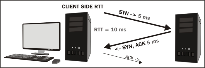
In a server-side capture, the time from the SYN, ACK to the client's ACK (third packet in the three-way handshake), also reflects the RTT. In practice, from any capture point, the time from the first SYN packet to the third ACK packet is a good representation of the RTT as well assuming the client and server response times during the handshake process are small. Be aware that the server response time to a SYN packet, while usually short, can be longer than normal during periods of high loading and can affect this measurement.
High network path latency isn't an error condition by itself, but can obviously have adverse effects on the application's operation over the network as previously discussed.
Bandwidth congestion affects the application's performance by extending the amount of time required to transmit a given amount of data over a network path; for users accessing an application server over a busy WAN link, these effects can become significant. A network support team should be able to generate bandwidth usage and availability reports for the in-path WAN links to check for this possibility, but you can also look for evidence of bandwidth congestion by using a properly configured Wireshark IO Graph to view network throughput during larger data transfers.
The following screenshot illustrates a data transfer that is affected by limited bandwidth; the flatlining at the 2.5 Mbps mark (the total bandwidth availability in this example), because no more bandwidth is available to support a faster transfer is clearly visible:

You can determine the peak data transfer rate in bits-per-second (bps) from an IO Graph by configuring the graph as follows:
- X Axis Tick interval: 1 sec
- Y Axis Unit: Bits/tick
- Graph 2 Filter:
ip.dst == <IP address of server> - Graph 4 Filter:
ip.src == <IP address of server>
These settings result in an accurate bits-per-second display of network throughput in client-to-server (red color) and server-to-client (blue color) directions. The Pixels per tick option in the X Axis panel, the Scale option in the Y Axis panel, and other settings can be modified as desired for the best display without affecting the accuracy of the measurement.
Be aware that most modern applications can generate short-term peak bandwidth demands (over an unrestricted link) of multiple Mbps. The WAN links along a network path should have enough spare capacity to accommodate these short term demands or response time will suffer accordingly. This is an important performance consideration.
There are a number of TCP data transport effects that can affect application performance; these can be analyzed in Wireshark.
Wireshark provides TCP StreamGraphs to analyze several key data transport metrics, including:
- Round-trip time: This graphs the RTT from a data packet to the corresponding ACK packet.
- Throughput: These are plots throughput in bytes per second.
- Time/sequence (Stephen's-style): This visualizes the TCP-based packet sequence numbers (and the number of bytes transferred) over time. An ideal graph flows from bottom-left to upper-right in a smooth fashion.
- Time/sequence (tcptrace): This is similar to the Stephen's graph, but provides more information. The data packets are represented with an I-bar display, where the taller the I-bar, the more data is being sent. A gray bar is also displayed that represents the receive window size. When the gray bar moves closer to the I-bars, the receive window size decreases.
- Window Scaling: This plots the receive window size.
These analysis graphs can be utilized by selecting one of the packets in a TCP stream in the Packet List pane and selecting TCP StreamGraph from the Statistics menu and then one of the options such as the Time-Sequence Graph (tcptrace).
The selected graph and Control Window will appear from the Graph type tab of the Control Window that you can select one of the other types of analysis graphs, as shown in the following screenshot:
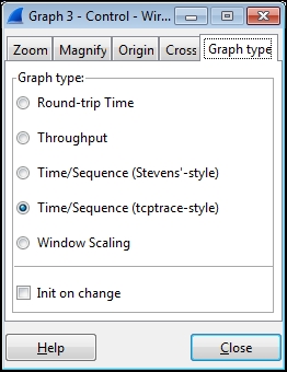
The Time/Sequence Graph (tcptrace) shown in the following screenshot plots sequence numbers as they increase during a data transfer, along with the gray receive window size line:
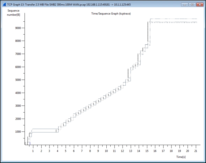
You can click and drag the mouse over a section of the graph to zoom into a particular section, or press the + key to zoom in and the - key to zoom out. Clicking on a point in any of the graphs will take you to the corresponding packet in the Wireshark's Packet List pane.
You can also analyze a the effects of TCP issues on network throughput by applying TCP analysis display filter strings to Wireshark's IO Graph, such as:
tcp.analysis.flags && !tcp.analysis.window_update
In the following screenshot of a slow SMB data transfer, it can be seen that the multiple TCP issues (in this case, packet loss, Duplicate ACKs, and retransmissions) in the red line correspond to a decrease in throughput (the black line):

Clicking on a point in the IO Graph takes you to the corresponding packet in the Wireshark's Packet List pane so you can investigate the issue.
Wireshark 2.0, also known as Wireshark Qt, is a major change in Wireshark's version history due to a transition from the GTK+ user interface library to Qt to provide better ongoing UI coverage for the supported platforms. Most of the Wireshark features and user interface controls will remain basically the same, but there are changes to the IO Graph.
These are shown in the following screenshot, which shows the same TCP issues that were seen in the preceding screenshot:
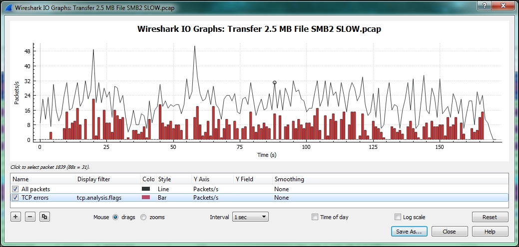
The new IO Graph window features the ability to add as many lines as desired (using the + key) and to zoom in on a graph line, as well as the ability to save the graph as an image or PDF document.
Top five reasons for poor application performance
Generally speaking, performance issues can be attributed to one of the following five areas, in order of decreasing likelihood:
- Server processing time delay
- Application turns delay
- Network path latency
- Bandwidth congestion
- Data transport (TCP) issues
Client processing time is usually a relatively small component of overall response time—except perhaps for some compute-extensive desktop applications, which leaves the focus on the network and server environments and any performance-affecting application design characteristics.
As was done when preparing to troubleshoot a connectivity or functionality problem, you'll need to gather the right information about the application environment and problem domain. You'll also want to determine which tools you may need to use during the analysis: Wireshark, TAPs to facilitate packet captures, and any other analysis tools.
You will also need to determine where to perform the first packet capture:
- A client-side capture is the best place to begin a performance analysis effort. From this vantage point, you can view and verify what the user is complaining about, view any error messages presented to the user or evident in the packet capture, measure network round-trip times, and capture the performance characteristics to study within a packet capture without the need to use a capture filter so you know you won't miss anything.
- A server-side capture may be needed because a client-side capture may not be possible for a user that is at a long distance, or to analyze server-to-server transactions to backend databases or other data sources.
- A packet capture at some intermediate point in the network path may be needed to isolate the source of excessive packet loss/errors and the associated retransmissions.
Remember that the use of an aggregating TAP is preferable over using SPAN ports, or you can install Wireshark on the client workstation or server as a last resort, but get the capture done any way you have to.
After performing the capture and saving the bulk capture file, confirm the following:
- Check the file to ensure there are no packets with the ACKed Unseen Segment messages in the Wireshark Warnings tab in the Expert Info menu, which means Wireshark saw a packet that was acknowledged but didn't see the original packet; an indication that Wireshark is missing packets due to a bad TAP or SPAN port configuration or excessive traffic levels. In any case, if more than just a few of these show up, you'll want to do the capture again after confirming the capture setup.
- Next, you'll want to review the captured conversations in IPv4 in the Conversations window and sort the Bytes column. The IP conversation between the user and application server should be at or near the top so you can select this conversation, right-click on it, and select A <-> B in the Selected menu.
- After reviewing the filtered data to ensure it contains what you expected, select Export Specified Packets from the File menu and save the filtered capture file with a filename that reflects the fact that this is a filtered subset of the bulk capture file.
- Finally, open the filtered file you just saved so you're working with a smaller, faster file without any distracting packets from other conversations that have nothing to do with your analysis.
At the onset of your analysis, you should take a look through the Errors, Warnings, and Notes tabs of Wireshark's Expert Info window (Analyze | Expert Info) for significant errors such as excessive retransmissions, Zero Window conditions, or application errors. These are very helpful to provide clues to the source of reported poor performance.
Although a few lost packets and retransmissions are normal and of minimal consequence in most packet captures, an excessive number indicates that network congestion is occurring somewhere in the path between user and server, packets are being discarded, and that an appreciable amount of time may be lost recovering from these lost packets.
Seeing a high count number of Duplicate ACK packets in the Expert Info Notes window may be alarming, but can be misleading. In the following screenshot, there was up to 69 Duplicate ACKs for one lost packet, and for a second lost packet the count went up to 89 (not shown in the following screenshot):
However, upon marking the time when the first Duplicate ACK occurred in Wireshark using the Set/Unset Time Reference feature in the Edit menu and then going to the last Duplicate ACK in this series by clicking the packet number in the Expert Info screen and inspecting a Relative time column in the Packet List pane, only 30 milliseconds had transpired. This is not a significant amount of time, especially if Selective Acknowledgment is enabled (as it was in this example) and other packets are being delivered and acknowledged in the meantime. Over longer latency network paths, the Duplicate ACK count can go much higher; it's only when the total number of lost packets and required retransmissions gets excessively high that the delay may become noticeable to a user.
Another condition to look for in the Expert Info Notes window includes the TCP Zero Window reports, which are caused by a receive buffer on the client or server being too full to accept any more data until the application has time to retrieve and process the data and make more room in the buffer. This isn't necessarily an error condition, but it can lead to substantial delays in transferring data, depending on how long it takes the buffer to get relieved.
You can measure this time by marking the TCP Zero Window packet with a time reference and looking at the elapsed relative time until a TCP Window Update packet is sent, which indicates the receiver is ready for more data. If this occurs frequently, or the delay between Zero Window and Window Update packets is long, you may need to inspect the host that is experiencing the full buffer condition to see whether there are any background processes that are adversely affecting the application that you're analyzing.
Note
If you haven't added them already, you need to add the Relative time and Delta time columns in the Packet List pane. Navigate to Edit | Preferences | Columns to add these. Adding time columns was also explained in Chapter 4, Configuring Wireshark.
You will probably see the connection reset (RST) messages in the Warnings tab. These are not indicators of an error condition if they occur at the end of a client-server exchange or session; they are normal indicators of sessions being terminated.
A very handy Filter Expression button you may want to add to Wireshark is a TCP Issues button using this display filter string as follows:
tcp.analysis.flags && !tcp.analysis.window_update && !tcp.analysis.keep_alive && !tcp.analysis.keep_alive_ack
This will filter and display most of the packets for which you will see the messages in the Expert Info window and provide a quick overview of any significant issues.
Since we're addressing application performance, the first step is to identify any delays in the packet flow so we can focus on the surrounding packets to identify the source and nature of the delay.
One of the quickest ways to identify delay events is to sort a TCP Delta time column (by clicking on the column header) so that the highest delay packets are arranged at the top of the packet list. You can then inspect the Info field of these packets to determine which, if any, reflect a valid performance affecting the event as most of them do not.
In the following screenshot, a TCP Delta time column is sorted in order of descending inter-packet times:
Let's have a detailed look at all the packets:
- The first two packets are the TCP Keep-Alive packets, which do just what they're called. They are a way for the client (or server) to make sure a connection is still alive (and not broken because the other end has gone away) after some time has elapsed with no activity. You can disregard these; they usually have nothing to do with the user experience.
- The third packet is a Reset packet, which is the last packet in the conversation stream and was sent to terminate the connection. Again, it has no impact on the user experience so you can ignore this.
- The next series of packets listed with a high inter-packet delay were GETs and a POST. These are the start of a new request and have occurred because the user clicked on a button or some other action on the application. However, the time that expired before these packets appear were consumed by the user think time—a period when the user was reading the last page and deciding what to do next. These also did not affect the user's response time experience and can be disregarded.
- Finally, Frame # 3691, which is a HTTP/1.1 200 OK, is a response from the server to a previous request; this is a legitimate response time of 1.9 seconds during which the user was waiting. If this response time had consumed more than a few seconds, the user may have grown frustrated with the wait and the type of request and reason for the excessive delay would warrant further analysis to determine why it took so long.
The point of this discussion is to illustrate that not all delays you may see in a packet trace affect the end user experience; you have to locate and focus on just those that do.
You may want to add some extra columns to Wireshark to speed up the analysis process; you can right-click on a column header and select Hide Column or Displayed Columns to show or hide specific columns:
- TCP Delta (tcp.time_delta): This is the time from one packet in a TCP conversation to the next packet in the same conversation/stream
- DNS Delta (dns.time): This is the time between DNS requests and responses
- HTTP Delta (http.time): This is the time between the HTTP requests and responses
While you're adding columns, the following can also be helpful during a performance analysis:
- Stream # (tcp.stream): This is the TCP conversation stream number. You can right-click on a stream number in this column, and select Selected from the Apply as a filter menu to quickly build a display filter to inspect a single conversation.
- Calc Win Size (tcp.window_size): This is the calculated TCP window size. This column can be used to quickly spot periods within a data delivery flow when the buffer size is decreasing to the point where a Zero Window condition occurred or almost occurred.
One of the most common causes of poor response times are excessively long server processing time events, which can be caused by processing times on the application server itself and/or delays incurred from long response times from a high number of requests to backend databases or other data sources.
Confirming and measuring these response times is easy within Wireshark using the following approach:
- Having used the sorted Delta Time column approach discussed in the previous section to identify a legitimate response time event, click on the suspect packet and then click on the Delta Time column header until it is no longer in the sort mode. This should result in the selected packet being highlighted in the middle of the Packet List pane and the displayed packets are back in their original order.
- Inspect the previous several packets to find the request that resulted in the long response time. The pattern that you'll see time and again is:
- The user sends a request to the server.
- The server fairly quickly acknowledges the request (with a [ACK] packet).
- After some time, the server starts sending data packets to service the request; the first of these packets is the packet you saw and selected in the sorted Delta Time view.
The time that expires between the first user request packet and the third packet when the server actually starts sending data is the First Byte response time. This is the area where you'll see longer response times caused by server processing time. This effect can be seen between users and servers, as well as between application servers and database servers or other data sources.
In the following screenshot, you can see a GET request from the client followed by an ACK packet from the server 198 milliseconds later (0.198651 seconds in the Delta Time Displ column); 1.9 seconds after that the server sends the first data packet (HTTP/1.1 200 OK in the Info field) followed by the start of a series of additional packets to deliver all of the requested data. In this illustration, a Time Reference has been set on the request packet. Looking at the Rel Time column, it can be seen that 2.107481 seconds transpired between the original request packet and the first byte packet:
It should be noted that how the First Byte data packet is summarized in the Info field depends upon the state of the Allow subdissector to reassemble TCP streams setting in the TCP menu, which can be found by navigating to Edit | Preferences | Protocols, as follows:
- If this option is disabled, the First Byte packet will display a summary of the contents of the first data packet in the Info field, such as HTTP/1.1 200 OK shown in the preceding screenshot, followed by a series of data delivery packets. The end of this delivery process has no remarkable signature; the packet flow just stops until the next request is received.
- If the Allow subdissector to reassemble TCP streams option is enabled, the First Byte packet will be summarized as simply a TCP segment of a reassembled PDU or similar notation. The HTTP/1.1 200 OK summary will be displayed in the Info field of the last data packet in this delivery process, signifying that the requested data has been delivered. An example of having this option enabled is illustrated in the following screenshot. This is the same request/response stream as shown in the preceding screenshot. It can be seen in the Rel Time column that the total elapsed time from the original request to the last data delivery packet was 2.1097 seconds:
In either case, the total response time as experienced by the user will be the time that transpires from the client request packet to the end of the data delivery packet plus the (usually) small amount of time required for the client application to process the received data and display the results on the user's screen.
In summary, measuring the time from the first request to the First Byte packets is the server response time. The time from the first request packet to the final data delivery packet is a good representation of the user response time experience.
The next, most likely source of poor response times—especially for remote users accessing applications over longer distances—is a relatively high number of what is known as application turns. An app turn is an instance where a client application makes a request and nothing else can or does happen until the response is received, after which another request/response cycle can occur, and so on.
Every client/server application is subject to the application turn effects and every request/response cycle incurs one. An application that imposes a high number of app turns to complete a task—due to poor application design, usually—can subject an end user to poor response times over higher latency network paths as the time spent waiting for these multiple requests and responses to traverse back and forth across the network adds up, which it can do quickly.
For example, if an application requires 100 application turns to complete a task and the round trip time (RTT) between the user and the application is 50 milliseconds (a typical cross-country value), the app turns delay will be 5 seconds:
100 App Turns X 50 ms RTT network latency = 5 seconds
This app turns' effect is additional wait (response) time on top of any server processing and network transport delays that is 5 seconds of totally wasted time. The resultant longer time inevitably gets blamed on the network; the network support teams assert that the network is working just fine and the application team points out that the application works fine until the network gets involved. And on it goes, so it is important to know about the app turns effects, what causes them, and how to measure and account for them.
Web applications can incur a relatively high app turn count due to the need to download one or more CSS files, JavaScript files, and multiple images to populate a page. Web designers can use techniques to reduce the app turn and download times, and modern browsers allow numerous connections to be used at the same time so that multiple requests can be serviced simultaneously, but the effects can still be significant over longer network paths. Many older, legacy applications and Microsoft's Server Message Block (SMB) protocols are also known to impose a high app turn count.
The presence and effects of application turns are not intuitively apparent in a packet capture unless you know they exist and how to identify and count them. You can do this in Wireshark for a client-side capture using a display filter:
ip.scr == 10.1.1.125 && tcp.analysis.ack_rtt > .008 && tcp.flags.ack == 1
You will need to replace the ip.src IP address with that of your server, and adjust the tcp.analysis.ack_rtt value to the RTT of the network path between the user and server. Upon applying the filter, you will see a display of packets that represent an application turn, and you can see the total app turns count in the Displayed field in the center section of the Wireshark's Status Bar option at the bottom of the user interface.
If you measure the total time required to complete a task (first request packet to last data delivery packet) and divide that time into the time incurred for application turns (number of app turns X network RTT), you can derive an approximate app turn time percentage:
5 seconds app turns delay / 7.5 seconds total response time = 66% of RT
Any percentage over 25 percent warrants further investigation into what can be done to reduce either the RTT latency (server placement) or the number app turns (application design).
The next leading cause of high response times is network path latency, which compounds the effects of application turns as discussed in the preceding section, as well as affecting data transport throughput and how long it takes to recover from packet loss and the subsequent retransmissions.
You can measure the network path latency between a client and server using the ICMP ping packets, but you can also determine this delay from a packet capture by measuring the time that transpires from a client SYN packet to the server's SYN, ACK response during a TCP three-way handshake process, as illustrated in the following figure of a client-side capture:
In a server-side capture, the time from the SYN, ACK to the client's ACK (third packet in the three-way handshake), also reflects the RTT. In practice, from any capture point, the time from the first SYN packet to the third ACK packet is a good representation of the RTT as well assuming the client and server response times during the handshake process are small. Be aware that the server response time to a SYN packet, while usually short, can be longer than normal during periods of high loading and can affect this measurement.
High network path latency isn't an error condition by itself, but can obviously have adverse effects on the application's operation over the network as previously discussed.
Bandwidth congestion affects the application's performance by extending the amount of time required to transmit a given amount of data over a network path; for users accessing an application server over a busy WAN link, these effects can become significant. A network support team should be able to generate bandwidth usage and availability reports for the in-path WAN links to check for this possibility, but you can also look for evidence of bandwidth congestion by using a properly configured Wireshark IO Graph to view network throughput during larger data transfers.
The following screenshot illustrates a data transfer that is affected by limited bandwidth; the flatlining at the 2.5 Mbps mark (the total bandwidth availability in this example), because no more bandwidth is available to support a faster transfer is clearly visible:
You can determine the peak data transfer rate in bits-per-second (bps) from an IO Graph by configuring the graph as follows:
- X Axis Tick interval: 1 sec
- Y Axis Unit: Bits/tick
- Graph 2 Filter:
ip.dst == <IP address of server> - Graph 4 Filter:
ip.src == <IP address of server>
These settings result in an accurate bits-per-second display of network throughput in client-to-server (red color) and server-to-client (blue color) directions. The Pixels per tick option in the X Axis panel, the Scale option in the Y Axis panel, and other settings can be modified as desired for the best display without affecting the accuracy of the measurement.
Be aware that most modern applications can generate short-term peak bandwidth demands (over an unrestricted link) of multiple Mbps. The WAN links along a network path should have enough spare capacity to accommodate these short term demands or response time will suffer accordingly. This is an important performance consideration.
There are a number of TCP data transport effects that can affect application performance; these can be analyzed in Wireshark.
Wireshark provides TCP StreamGraphs to analyze several key data transport metrics, including:
- Round-trip time: This graphs the RTT from a data packet to the corresponding ACK packet.
- Throughput: These are plots throughput in bytes per second.
- Time/sequence (Stephen's-style): This visualizes the TCP-based packet sequence numbers (and the number of bytes transferred) over time. An ideal graph flows from bottom-left to upper-right in a smooth fashion.
- Time/sequence (tcptrace): This is similar to the Stephen's graph, but provides more information. The data packets are represented with an I-bar display, where the taller the I-bar, the more data is being sent. A gray bar is also displayed that represents the receive window size. When the gray bar moves closer to the I-bars, the receive window size decreases.
- Window Scaling: This plots the receive window size.
These analysis graphs can be utilized by selecting one of the packets in a TCP stream in the Packet List pane and selecting TCP StreamGraph from the Statistics menu and then one of the options such as the Time-Sequence Graph (tcptrace).
The selected graph and Control Window will appear from the Graph type tab of the Control Window that you can select one of the other types of analysis graphs, as shown in the following screenshot:
The Time/Sequence Graph (tcptrace) shown in the following screenshot plots sequence numbers as they increase during a data transfer, along with the gray receive window size line:
You can click and drag the mouse over a section of the graph to zoom into a particular section, or press the + key to zoom in and the - key to zoom out. Clicking on a point in any of the graphs will take you to the corresponding packet in the Wireshark's Packet List pane.
You can also analyze a the effects of TCP issues on network throughput by applying TCP analysis display filter strings to Wireshark's IO Graph, such as:
tcp.analysis.flags && !tcp.analysis.window_update
In the following screenshot of a slow SMB data transfer, it can be seen that the multiple TCP issues (in this case, packet loss, Duplicate ACKs, and retransmissions) in the red line correspond to a decrease in throughput (the black line):
Clicking on a point in the IO Graph takes you to the corresponding packet in the Wireshark's Packet List pane so you can investigate the issue.
Wireshark 2.0, also known as Wireshark Qt, is a major change in Wireshark's version history due to a transition from the GTK+ user interface library to Qt to provide better ongoing UI coverage for the supported platforms. Most of the Wireshark features and user interface controls will remain basically the same, but there are changes to the IO Graph.
These are shown in the following screenshot, which shows the same TCP issues that were seen in the preceding screenshot:
The new IO Graph window features the ability to add as many lines as desired (using the + key) and to zoom in on a graph line, as well as the ability to save the graph as an image or PDF document.
Preparing the tools and approach
As was done when preparing to troubleshoot a connectivity or functionality problem, you'll need to gather the right information about the application environment and problem domain. You'll also want to determine which tools you may need to use during the analysis: Wireshark, TAPs to facilitate packet captures, and any other analysis tools.
You will also need to determine where to perform the first packet capture:
- A client-side capture is the best place to begin a performance analysis effort. From this vantage point, you can view and verify what the user is complaining about, view any error messages presented to the user or evident in the packet capture, measure network round-trip times, and capture the performance characteristics to study within a packet capture without the need to use a capture filter so you know you won't miss anything.
- A server-side capture may be needed because a client-side capture may not be possible for a user that is at a long distance, or to analyze server-to-server transactions to backend databases or other data sources.
- A packet capture at some intermediate point in the network path may be needed to isolate the source of excessive packet loss/errors and the associated retransmissions.
Remember that the use of an aggregating TAP is preferable over using SPAN ports, or you can install Wireshark on the client workstation or server as a last resort, but get the capture done any way you have to.
After performing the capture and saving the bulk capture file, confirm the following:
- Check the file to ensure there are no packets with the ACKed Unseen Segment messages in the Wireshark Warnings tab in the Expert Info menu, which means Wireshark saw a packet that was acknowledged but didn't see the original packet; an indication that Wireshark is missing packets due to a bad TAP or SPAN port configuration or excessive traffic levels. In any case, if more than just a few of these show up, you'll want to do the capture again after confirming the capture setup.
- Next, you'll want to review the captured conversations in IPv4 in the Conversations window and sort the Bytes column. The IP conversation between the user and application server should be at or near the top so you can select this conversation, right-click on it, and select A <-> B in the Selected menu.
- After reviewing the filtered data to ensure it contains what you expected, select Export Specified Packets from the File menu and save the filtered capture file with a filename that reflects the fact that this is a filtered subset of the bulk capture file.
- Finally, open the filtered file you just saved so you're working with a smaller, faster file without any distracting packets from other conversations that have nothing to do with your analysis.
At the onset of your analysis, you should take a look through the Errors, Warnings, and Notes tabs of Wireshark's Expert Info window (Analyze | Expert Info) for significant errors such as excessive retransmissions, Zero Window conditions, or application errors. These are very helpful to provide clues to the source of reported poor performance.
Although a few lost packets and retransmissions are normal and of minimal consequence in most packet captures, an excessive number indicates that network congestion is occurring somewhere in the path between user and server, packets are being discarded, and that an appreciable amount of time may be lost recovering from these lost packets.
Seeing a high count number of Duplicate ACK packets in the Expert Info Notes window may be alarming, but can be misleading. In the following screenshot, there was up to 69 Duplicate ACKs for one lost packet, and for a second lost packet the count went up to 89 (not shown in the following screenshot):
However, upon marking the time when the first Duplicate ACK occurred in Wireshark using the Set/Unset Time Reference feature in the Edit menu and then going to the last Duplicate ACK in this series by clicking the packet number in the Expert Info screen and inspecting a Relative time column in the Packet List pane, only 30 milliseconds had transpired. This is not a significant amount of time, especially if Selective Acknowledgment is enabled (as it was in this example) and other packets are being delivered and acknowledged in the meantime. Over longer latency network paths, the Duplicate ACK count can go much higher; it's only when the total number of lost packets and required retransmissions gets excessively high that the delay may become noticeable to a user.
Another condition to look for in the Expert Info Notes window includes the TCP Zero Window reports, which are caused by a receive buffer on the client or server being too full to accept any more data until the application has time to retrieve and process the data and make more room in the buffer. This isn't necessarily an error condition, but it can lead to substantial delays in transferring data, depending on how long it takes the buffer to get relieved.
You can measure this time by marking the TCP Zero Window packet with a time reference and looking at the elapsed relative time until a TCP Window Update packet is sent, which indicates the receiver is ready for more data. If this occurs frequently, or the delay between Zero Window and Window Update packets is long, you may need to inspect the host that is experiencing the full buffer condition to see whether there are any background processes that are adversely affecting the application that you're analyzing.
Note
If you haven't added them already, you need to add the Relative time and Delta time columns in the Packet List pane. Navigate to Edit | Preferences | Columns to add these. Adding time columns was also explained in Chapter 4, Configuring Wireshark.
You will probably see the connection reset (RST) messages in the Warnings tab. These are not indicators of an error condition if they occur at the end of a client-server exchange or session; they are normal indicators of sessions being terminated.
A very handy Filter Expression button you may want to add to Wireshark is a TCP Issues button using this display filter string as follows:
tcp.analysis.flags && !tcp.analysis.window_update && !tcp.analysis.keep_alive && !tcp.analysis.keep_alive_ack
This will filter and display most of the packets for which you will see the messages in the Expert Info window and provide a quick overview of any significant issues.
Since we're addressing application performance, the first step is to identify any delays in the packet flow so we can focus on the surrounding packets to identify the source and nature of the delay.
One of the quickest ways to identify delay events is to sort a TCP Delta time column (by clicking on the column header) so that the highest delay packets are arranged at the top of the packet list. You can then inspect the Info field of these packets to determine which, if any, reflect a valid performance affecting the event as most of them do not.
In the following screenshot, a TCP Delta time column is sorted in order of descending inter-packet times:
Let's have a detailed look at all the packets:
- The first two packets are the TCP Keep-Alive packets, which do just what they're called. They are a way for the client (or server) to make sure a connection is still alive (and not broken because the other end has gone away) after some time has elapsed with no activity. You can disregard these; they usually have nothing to do with the user experience.
- The third packet is a Reset packet, which is the last packet in the conversation stream and was sent to terminate the connection. Again, it has no impact on the user experience so you can ignore this.
- The next series of packets listed with a high inter-packet delay were GETs and a POST. These are the start of a new request and have occurred because the user clicked on a button or some other action on the application. However, the time that expired before these packets appear were consumed by the user think time—a period when the user was reading the last page and deciding what to do next. These also did not affect the user's response time experience and can be disregarded.
- Finally, Frame # 3691, which is a HTTP/1.1 200 OK, is a response from the server to a previous request; this is a legitimate response time of 1.9 seconds during which the user was waiting. If this response time had consumed more than a few seconds, the user may have grown frustrated with the wait and the type of request and reason for the excessive delay would warrant further analysis to determine why it took so long.
The point of this discussion is to illustrate that not all delays you may see in a packet trace affect the end user experience; you have to locate and focus on just those that do.
You may want to add some extra columns to Wireshark to speed up the analysis process; you can right-click on a column header and select Hide Column or Displayed Columns to show or hide specific columns:
- TCP Delta (tcp.time_delta): This is the time from one packet in a TCP conversation to the next packet in the same conversation/stream
- DNS Delta (dns.time): This is the time between DNS requests and responses
- HTTP Delta (http.time): This is the time between the HTTP requests and responses
While you're adding columns, the following can also be helpful during a performance analysis:
- Stream # (tcp.stream): This is the TCP conversation stream number. You can right-click on a stream number in this column, and select Selected from the Apply as a filter menu to quickly build a display filter to inspect a single conversation.
- Calc Win Size (tcp.window_size): This is the calculated TCP window size. This column can be used to quickly spot periods within a data delivery flow when the buffer size is decreasing to the point where a Zero Window condition occurred or almost occurred.
One of the most common causes of poor response times are excessively long server processing time events, which can be caused by processing times on the application server itself and/or delays incurred from long response times from a high number of requests to backend databases or other data sources.
Confirming and measuring these response times is easy within Wireshark using the following approach:
- Having used the sorted Delta Time column approach discussed in the previous section to identify a legitimate response time event, click on the suspect packet and then click on the Delta Time column header until it is no longer in the sort mode. This should result in the selected packet being highlighted in the middle of the Packet List pane and the displayed packets are back in their original order.
- Inspect the previous several packets to find the request that resulted in the long response time. The pattern that you'll see time and again is:
- The user sends a request to the server.
- The server fairly quickly acknowledges the request (with a [ACK] packet).
- After some time, the server starts sending data packets to service the request; the first of these packets is the packet you saw and selected in the sorted Delta Time view.
The time that expires between the first user request packet and the third packet when the server actually starts sending data is the First Byte response time. This is the area where you'll see longer response times caused by server processing time. This effect can be seen between users and servers, as well as between application servers and database servers or other data sources.
In the following screenshot, you can see a GET request from the client followed by an ACK packet from the server 198 milliseconds later (0.198651 seconds in the Delta Time Displ column); 1.9 seconds after that the server sends the first data packet (HTTP/1.1 200 OK in the Info field) followed by the start of a series of additional packets to deliver all of the requested data. In this illustration, a Time Reference has been set on the request packet. Looking at the Rel Time column, it can be seen that 2.107481 seconds transpired between the original request packet and the first byte packet:
It should be noted that how the First Byte data packet is summarized in the Info field depends upon the state of the Allow subdissector to reassemble TCP streams setting in the TCP menu, which can be found by navigating to Edit | Preferences | Protocols, as follows:
- If this option is disabled, the First Byte packet will display a summary of the contents of the first data packet in the Info field, such as HTTP/1.1 200 OK shown in the preceding screenshot, followed by a series of data delivery packets. The end of this delivery process has no remarkable signature; the packet flow just stops until the next request is received.
- If the Allow subdissector to reassemble TCP streams option is enabled, the First Byte packet will be summarized as simply a TCP segment of a reassembled PDU or similar notation. The HTTP/1.1 200 OK summary will be displayed in the Info field of the last data packet in this delivery process, signifying that the requested data has been delivered. An example of having this option enabled is illustrated in the following screenshot. This is the same request/response stream as shown in the preceding screenshot. It can be seen in the Rel Time column that the total elapsed time from the original request to the last data delivery packet was 2.1097 seconds:
In either case, the total response time as experienced by the user will be the time that transpires from the client request packet to the end of the data delivery packet plus the (usually) small amount of time required for the client application to process the received data and display the results on the user's screen.
In summary, measuring the time from the first request to the First Byte packets is the server response time. The time from the first request packet to the final data delivery packet is a good representation of the user response time experience.
The next, most likely source of poor response times—especially for remote users accessing applications over longer distances—is a relatively high number of what is known as application turns. An app turn is an instance where a client application makes a request and nothing else can or does happen until the response is received, after which another request/response cycle can occur, and so on.
Every client/server application is subject to the application turn effects and every request/response cycle incurs one. An application that imposes a high number of app turns to complete a task—due to poor application design, usually—can subject an end user to poor response times over higher latency network paths as the time spent waiting for these multiple requests and responses to traverse back and forth across the network adds up, which it can do quickly.
For example, if an application requires 100 application turns to complete a task and the round trip time (RTT) between the user and the application is 50 milliseconds (a typical cross-country value), the app turns delay will be 5 seconds:
100 App Turns X 50 ms RTT network latency = 5 seconds
This app turns' effect is additional wait (response) time on top of any server processing and network transport delays that is 5 seconds of totally wasted time. The resultant longer time inevitably gets blamed on the network; the network support teams assert that the network is working just fine and the application team points out that the application works fine until the network gets involved. And on it goes, so it is important to know about the app turns effects, what causes them, and how to measure and account for them.
Web applications can incur a relatively high app turn count due to the need to download one or more CSS files, JavaScript files, and multiple images to populate a page. Web designers can use techniques to reduce the app turn and download times, and modern browsers allow numerous connections to be used at the same time so that multiple requests can be serviced simultaneously, but the effects can still be significant over longer network paths. Many older, legacy applications and Microsoft's Server Message Block (SMB) protocols are also known to impose a high app turn count.
The presence and effects of application turns are not intuitively apparent in a packet capture unless you know they exist and how to identify and count them. You can do this in Wireshark for a client-side capture using a display filter:
ip.scr == 10.1.1.125 && tcp.analysis.ack_rtt > .008 && tcp.flags.ack == 1
You will need to replace the ip.src IP address with that of your server, and adjust the tcp.analysis.ack_rtt value to the RTT of the network path between the user and server. Upon applying the filter, you will see a display of packets that represent an application turn, and you can see the total app turns count in the Displayed field in the center section of the Wireshark's Status Bar option at the bottom of the user interface.
If you measure the total time required to complete a task (first request packet to last data delivery packet) and divide that time into the time incurred for application turns (number of app turns X network RTT), you can derive an approximate app turn time percentage:
5 seconds app turns delay / 7.5 seconds total response time = 66% of RT
Any percentage over 25 percent warrants further investigation into what can be done to reduce either the RTT latency (server placement) or the number app turns (application design).
The next leading cause of high response times is network path latency, which compounds the effects of application turns as discussed in the preceding section, as well as affecting data transport throughput and how long it takes to recover from packet loss and the subsequent retransmissions.
You can measure the network path latency between a client and server using the ICMP ping packets, but you can also determine this delay from a packet capture by measuring the time that transpires from a client SYN packet to the server's SYN, ACK response during a TCP three-way handshake process, as illustrated in the following figure of a client-side capture:
In a server-side capture, the time from the SYN, ACK to the client's ACK (third packet in the three-way handshake), also reflects the RTT. In practice, from any capture point, the time from the first SYN packet to the third ACK packet is a good representation of the RTT as well assuming the client and server response times during the handshake process are small. Be aware that the server response time to a SYN packet, while usually short, can be longer than normal during periods of high loading and can affect this measurement.
High network path latency isn't an error condition by itself, but can obviously have adverse effects on the application's operation over the network as previously discussed.
Bandwidth congestion affects the application's performance by extending the amount of time required to transmit a given amount of data over a network path; for users accessing an application server over a busy WAN link, these effects can become significant. A network support team should be able to generate bandwidth usage and availability reports for the in-path WAN links to check for this possibility, but you can also look for evidence of bandwidth congestion by using a properly configured Wireshark IO Graph to view network throughput during larger data transfers.
The following screenshot illustrates a data transfer that is affected by limited bandwidth; the flatlining at the 2.5 Mbps mark (the total bandwidth availability in this example), because no more bandwidth is available to support a faster transfer is clearly visible:
You can determine the peak data transfer rate in bits-per-second (bps) from an IO Graph by configuring the graph as follows:
- X Axis Tick interval: 1 sec
- Y Axis Unit: Bits/tick
- Graph 2 Filter:
ip.dst == <IP address of server> - Graph 4 Filter:
ip.src == <IP address of server>
These settings result in an accurate bits-per-second display of network throughput in client-to-server (red color) and server-to-client (blue color) directions. The Pixels per tick option in the X Axis panel, the Scale option in the Y Axis panel, and other settings can be modified as desired for the best display without affecting the accuracy of the measurement.
Be aware that most modern applications can generate short-term peak bandwidth demands (over an unrestricted link) of multiple Mbps. The WAN links along a network path should have enough spare capacity to accommodate these short term demands or response time will suffer accordingly. This is an important performance consideration.
There are a number of TCP data transport effects that can affect application performance; these can be analyzed in Wireshark.
Wireshark provides TCP StreamGraphs to analyze several key data transport metrics, including:
- Round-trip time: This graphs the RTT from a data packet to the corresponding ACK packet.
- Throughput: These are plots throughput in bytes per second.
- Time/sequence (Stephen's-style): This visualizes the TCP-based packet sequence numbers (and the number of bytes transferred) over time. An ideal graph flows from bottom-left to upper-right in a smooth fashion.
- Time/sequence (tcptrace): This is similar to the Stephen's graph, but provides more information. The data packets are represented with an I-bar display, where the taller the I-bar, the more data is being sent. A gray bar is also displayed that represents the receive window size. When the gray bar moves closer to the I-bars, the receive window size decreases.
- Window Scaling: This plots the receive window size.
These analysis graphs can be utilized by selecting one of the packets in a TCP stream in the Packet List pane and selecting TCP StreamGraph from the Statistics menu and then one of the options such as the Time-Sequence Graph (tcptrace).
The selected graph and Control Window will appear from the Graph type tab of the Control Window that you can select one of the other types of analysis graphs, as shown in the following screenshot:
The Time/Sequence Graph (tcptrace) shown in the following screenshot plots sequence numbers as they increase during a data transfer, along with the gray receive window size line:
You can click and drag the mouse over a section of the graph to zoom into a particular section, or press the + key to zoom in and the - key to zoom out. Clicking on a point in any of the graphs will take you to the corresponding packet in the Wireshark's Packet List pane.
You can also analyze a the effects of TCP issues on network throughput by applying TCP analysis display filter strings to Wireshark's IO Graph, such as:
tcp.analysis.flags && !tcp.analysis.window_update
In the following screenshot of a slow SMB data transfer, it can be seen that the multiple TCP issues (in this case, packet loss, Duplicate ACKs, and retransmissions) in the red line correspond to a decrease in throughput (the black line):
Clicking on a point in the IO Graph takes you to the corresponding packet in the Wireshark's Packet List pane so you can investigate the issue.
Wireshark 2.0, also known as Wireshark Qt, is a major change in Wireshark's version history due to a transition from the GTK+ user interface library to Qt to provide better ongoing UI coverage for the supported platforms. Most of the Wireshark features and user interface controls will remain basically the same, but there are changes to the IO Graph.
These are shown in the following screenshot, which shows the same TCP issues that were seen in the preceding screenshot:
The new IO Graph window features the ability to add as many lines as desired (using the + key) and to zoom in on a graph line, as well as the ability to save the graph as an image or PDF document.
Performing, verifying, and saving a good packet capture
After performing the capture and saving the bulk capture file, confirm the following:
- Check the file to ensure there are no packets with the ACKed Unseen Segment messages in the Wireshark Warnings tab in the Expert Info menu, which means Wireshark saw a packet that was acknowledged but didn't see the original packet; an indication that Wireshark is missing packets due to a bad TAP or SPAN port configuration or excessive traffic levels. In any case, if more than just a few of these show up, you'll want to do the capture again after confirming the capture setup.
- Next, you'll want to review the captured conversations in IPv4 in the Conversations window and sort the Bytes column. The IP conversation between the user and application server should be at or near the top so you can select this conversation, right-click on it, and select A <-> B in the Selected menu.
- After reviewing the filtered data to ensure it contains what you expected, select Export Specified Packets from the File menu and save the filtered capture file with a filename that reflects the fact that this is a filtered subset of the bulk capture file.
- Finally, open the filtered file you just saved so you're working with a smaller, faster file without any distracting packets from other conversations that have nothing to do with your analysis.
At the onset of your analysis, you should take a look through the Errors, Warnings, and Notes tabs of Wireshark's Expert Info window (Analyze | Expert Info) for significant errors such as excessive retransmissions, Zero Window conditions, or application errors. These are very helpful to provide clues to the source of reported poor performance.
Although a few lost packets and retransmissions are normal and of minimal consequence in most packet captures, an excessive number indicates that network congestion is occurring somewhere in the path between user and server, packets are being discarded, and that an appreciable amount of time may be lost recovering from these lost packets.
Seeing a high count number of Duplicate ACK packets in the Expert Info Notes window may be alarming, but can be misleading. In the following screenshot, there was up to 69 Duplicate ACKs for one lost packet, and for a second lost packet the count went up to 89 (not shown in the following screenshot):
However, upon marking the time when the first Duplicate ACK occurred in Wireshark using the Set/Unset Time Reference feature in the Edit menu and then going to the last Duplicate ACK in this series by clicking the packet number in the Expert Info screen and inspecting a Relative time column in the Packet List pane, only 30 milliseconds had transpired. This is not a significant amount of time, especially if Selective Acknowledgment is enabled (as it was in this example) and other packets are being delivered and acknowledged in the meantime. Over longer latency network paths, the Duplicate ACK count can go much higher; it's only when the total number of lost packets and required retransmissions gets excessively high that the delay may become noticeable to a user.
Another condition to look for in the Expert Info Notes window includes the TCP Zero Window reports, which are caused by a receive buffer on the client or server being too full to accept any more data until the application has time to retrieve and process the data and make more room in the buffer. This isn't necessarily an error condition, but it can lead to substantial delays in transferring data, depending on how long it takes the buffer to get relieved.
You can measure this time by marking the TCP Zero Window packet with a time reference and looking at the elapsed relative time until a TCP Window Update packet is sent, which indicates the receiver is ready for more data. If this occurs frequently, or the delay between Zero Window and Window Update packets is long, you may need to inspect the host that is experiencing the full buffer condition to see whether there are any background processes that are adversely affecting the application that you're analyzing.
Note
If you haven't added them already, you need to add the Relative time and Delta time columns in the Packet List pane. Navigate to Edit | Preferences | Columns to add these. Adding time columns was also explained in Chapter 4, Configuring Wireshark.
You will probably see the connection reset (RST) messages in the Warnings tab. These are not indicators of an error condition if they occur at the end of a client-server exchange or session; they are normal indicators of sessions being terminated.
A very handy Filter Expression button you may want to add to Wireshark is a TCP Issues button using this display filter string as follows:
tcp.analysis.flags && !tcp.analysis.window_update && !tcp.analysis.keep_alive && !tcp.analysis.keep_alive_ack
This will filter and display most of the packets for which you will see the messages in the Expert Info window and provide a quick overview of any significant issues.
Since we're addressing application performance, the first step is to identify any delays in the packet flow so we can focus on the surrounding packets to identify the source and nature of the delay.
One of the quickest ways to identify delay events is to sort a TCP Delta time column (by clicking on the column header) so that the highest delay packets are arranged at the top of the packet list. You can then inspect the Info field of these packets to determine which, if any, reflect a valid performance affecting the event as most of them do not.
In the following screenshot, a TCP Delta time column is sorted in order of descending inter-packet times:
Let's have a detailed look at all the packets:
- The first two packets are the TCP Keep-Alive packets, which do just what they're called. They are a way for the client (or server) to make sure a connection is still alive (and not broken because the other end has gone away) after some time has elapsed with no activity. You can disregard these; they usually have nothing to do with the user experience.
- The third packet is a Reset packet, which is the last packet in the conversation stream and was sent to terminate the connection. Again, it has no impact on the user experience so you can ignore this.
- The next series of packets listed with a high inter-packet delay were GETs and a POST. These are the start of a new request and have occurred because the user clicked on a button or some other action on the application. However, the time that expired before these packets appear were consumed by the user think time—a period when the user was reading the last page and deciding what to do next. These also did not affect the user's response time experience and can be disregarded.
- Finally, Frame # 3691, which is a HTTP/1.1 200 OK, is a response from the server to a previous request; this is a legitimate response time of 1.9 seconds during which the user was waiting. If this response time had consumed more than a few seconds, the user may have grown frustrated with the wait and the type of request and reason for the excessive delay would warrant further analysis to determine why it took so long.
The point of this discussion is to illustrate that not all delays you may see in a packet trace affect the end user experience; you have to locate and focus on just those that do.
You may want to add some extra columns to Wireshark to speed up the analysis process; you can right-click on a column header and select Hide Column or Displayed Columns to show or hide specific columns:
- TCP Delta (tcp.time_delta): This is the time from one packet in a TCP conversation to the next packet in the same conversation/stream
- DNS Delta (dns.time): This is the time between DNS requests and responses
- HTTP Delta (http.time): This is the time between the HTTP requests and responses
While you're adding columns, the following can also be helpful during a performance analysis:
- Stream # (tcp.stream): This is the TCP conversation stream number. You can right-click on a stream number in this column, and select Selected from the Apply as a filter menu to quickly build a display filter to inspect a single conversation.
- Calc Win Size (tcp.window_size): This is the calculated TCP window size. This column can be used to quickly spot periods within a data delivery flow when the buffer size is decreasing to the point where a Zero Window condition occurred or almost occurred.
One of the most common causes of poor response times are excessively long server processing time events, which can be caused by processing times on the application server itself and/or delays incurred from long response times from a high number of requests to backend databases or other data sources.
Confirming and measuring these response times is easy within Wireshark using the following approach:
- Having used the sorted Delta Time column approach discussed in the previous section to identify a legitimate response time event, click on the suspect packet and then click on the Delta Time column header until it is no longer in the sort mode. This should result in the selected packet being highlighted in the middle of the Packet List pane and the displayed packets are back in their original order.
- Inspect the previous several packets to find the request that resulted in the long response time. The pattern that you'll see time and again is:
- The user sends a request to the server.
- The server fairly quickly acknowledges the request (with a [ACK] packet).
- After some time, the server starts sending data packets to service the request; the first of these packets is the packet you saw and selected in the sorted Delta Time view.
The time that expires between the first user request packet and the third packet when the server actually starts sending data is the First Byte response time. This is the area where you'll see longer response times caused by server processing time. This effect can be seen between users and servers, as well as between application servers and database servers or other data sources.
In the following screenshot, you can see a GET request from the client followed by an ACK packet from the server 198 milliseconds later (0.198651 seconds in the Delta Time Displ column); 1.9 seconds after that the server sends the first data packet (HTTP/1.1 200 OK in the Info field) followed by the start of a series of additional packets to deliver all of the requested data. In this illustration, a Time Reference has been set on the request packet. Looking at the Rel Time column, it can be seen that 2.107481 seconds transpired between the original request packet and the first byte packet:
It should be noted that how the First Byte data packet is summarized in the Info field depends upon the state of the Allow subdissector to reassemble TCP streams setting in the TCP menu, which can be found by navigating to Edit | Preferences | Protocols, as follows:
- If this option is disabled, the First Byte packet will display a summary of the contents of the first data packet in the Info field, such as HTTP/1.1 200 OK shown in the preceding screenshot, followed by a series of data delivery packets. The end of this delivery process has no remarkable signature; the packet flow just stops until the next request is received.
- If the Allow subdissector to reassemble TCP streams option is enabled, the First Byte packet will be summarized as simply a TCP segment of a reassembled PDU or similar notation. The HTTP/1.1 200 OK summary will be displayed in the Info field of the last data packet in this delivery process, signifying that the requested data has been delivered. An example of having this option enabled is illustrated in the following screenshot. This is the same request/response stream as shown in the preceding screenshot. It can be seen in the Rel Time column that the total elapsed time from the original request to the last data delivery packet was 2.1097 seconds:
In either case, the total response time as experienced by the user will be the time that transpires from the client request packet to the end of the data delivery packet plus the (usually) small amount of time required for the client application to process the received data and display the results on the user's screen.
In summary, measuring the time from the first request to the First Byte packets is the server response time. The time from the first request packet to the final data delivery packet is a good representation of the user response time experience.
The next, most likely source of poor response times—especially for remote users accessing applications over longer distances—is a relatively high number of what is known as application turns. An app turn is an instance where a client application makes a request and nothing else can or does happen until the response is received, after which another request/response cycle can occur, and so on.
Every client/server application is subject to the application turn effects and every request/response cycle incurs one. An application that imposes a high number of app turns to complete a task—due to poor application design, usually—can subject an end user to poor response times over higher latency network paths as the time spent waiting for these multiple requests and responses to traverse back and forth across the network adds up, which it can do quickly.
For example, if an application requires 100 application turns to complete a task and the round trip time (RTT) between the user and the application is 50 milliseconds (a typical cross-country value), the app turns delay will be 5 seconds:
100 App Turns X 50 ms RTT network latency = 5 seconds
This app turns' effect is additional wait (response) time on top of any server processing and network transport delays that is 5 seconds of totally wasted time. The resultant longer time inevitably gets blamed on the network; the network support teams assert that the network is working just fine and the application team points out that the application works fine until the network gets involved. And on it goes, so it is important to know about the app turns effects, what causes them, and how to measure and account for them.
Web applications can incur a relatively high app turn count due to the need to download one or more CSS files, JavaScript files, and multiple images to populate a page. Web designers can use techniques to reduce the app turn and download times, and modern browsers allow numerous connections to be used at the same time so that multiple requests can be serviced simultaneously, but the effects can still be significant over longer network paths. Many older, legacy applications and Microsoft's Server Message Block (SMB) protocols are also known to impose a high app turn count.
The presence and effects of application turns are not intuitively apparent in a packet capture unless you know they exist and how to identify and count them. You can do this in Wireshark for a client-side capture using a display filter:
ip.scr == 10.1.1.125 && tcp.analysis.ack_rtt > .008 && tcp.flags.ack == 1
You will need to replace the ip.src IP address with that of your server, and adjust the tcp.analysis.ack_rtt value to the RTT of the network path between the user and server. Upon applying the filter, you will see a display of packets that represent an application turn, and you can see the total app turns count in the Displayed field in the center section of the Wireshark's Status Bar option at the bottom of the user interface.
If you measure the total time required to complete a task (first request packet to last data delivery packet) and divide that time into the time incurred for application turns (number of app turns X network RTT), you can derive an approximate app turn time percentage:
5 seconds app turns delay / 7.5 seconds total response time = 66% of RT
Any percentage over 25 percent warrants further investigation into what can be done to reduce either the RTT latency (server placement) or the number app turns (application design).
The next leading cause of high response times is network path latency, which compounds the effects of application turns as discussed in the preceding section, as well as affecting data transport throughput and how long it takes to recover from packet loss and the subsequent retransmissions.
You can measure the network path latency between a client and server using the ICMP ping packets, but you can also determine this delay from a packet capture by measuring the time that transpires from a client SYN packet to the server's SYN, ACK response during a TCP three-way handshake process, as illustrated in the following figure of a client-side capture:
In a server-side capture, the time from the SYN, ACK to the client's ACK (third packet in the three-way handshake), also reflects the RTT. In practice, from any capture point, the time from the first SYN packet to the third ACK packet is a good representation of the RTT as well assuming the client and server response times during the handshake process are small. Be aware that the server response time to a SYN packet, while usually short, can be longer than normal during periods of high loading and can affect this measurement.
High network path latency isn't an error condition by itself, but can obviously have adverse effects on the application's operation over the network as previously discussed.
Bandwidth congestion affects the application's performance by extending the amount of time required to transmit a given amount of data over a network path; for users accessing an application server over a busy WAN link, these effects can become significant. A network support team should be able to generate bandwidth usage and availability reports for the in-path WAN links to check for this possibility, but you can also look for evidence of bandwidth congestion by using a properly configured Wireshark IO Graph to view network throughput during larger data transfers.
The following screenshot illustrates a data transfer that is affected by limited bandwidth; the flatlining at the 2.5 Mbps mark (the total bandwidth availability in this example), because no more bandwidth is available to support a faster transfer is clearly visible:
You can determine the peak data transfer rate in bits-per-second (bps) from an IO Graph by configuring the graph as follows:
- X Axis Tick interval: 1 sec
- Y Axis Unit: Bits/tick
- Graph 2 Filter:
ip.dst == <IP address of server> - Graph 4 Filter:
ip.src == <IP address of server>
These settings result in an accurate bits-per-second display of network throughput in client-to-server (red color) and server-to-client (blue color) directions. The Pixels per tick option in the X Axis panel, the Scale option in the Y Axis panel, and other settings can be modified as desired for the best display without affecting the accuracy of the measurement.
Be aware that most modern applications can generate short-term peak bandwidth demands (over an unrestricted link) of multiple Mbps. The WAN links along a network path should have enough spare capacity to accommodate these short term demands or response time will suffer accordingly. This is an important performance consideration.
There are a number of TCP data transport effects that can affect application performance; these can be analyzed in Wireshark.
Wireshark provides TCP StreamGraphs to analyze several key data transport metrics, including:
- Round-trip time: This graphs the RTT from a data packet to the corresponding ACK packet.
- Throughput: These are plots throughput in bytes per second.
- Time/sequence (Stephen's-style): This visualizes the TCP-based packet sequence numbers (and the number of bytes transferred) over time. An ideal graph flows from bottom-left to upper-right in a smooth fashion.
- Time/sequence (tcptrace): This is similar to the Stephen's graph, but provides more information. The data packets are represented with an I-bar display, where the taller the I-bar, the more data is being sent. A gray bar is also displayed that represents the receive window size. When the gray bar moves closer to the I-bars, the receive window size decreases.
- Window Scaling: This plots the receive window size.
These analysis graphs can be utilized by selecting one of the packets in a TCP stream in the Packet List pane and selecting TCP StreamGraph from the Statistics menu and then one of the options such as the Time-Sequence Graph (tcptrace).
The selected graph and Control Window will appear from the Graph type tab of the Control Window that you can select one of the other types of analysis graphs, as shown in the following screenshot:
The Time/Sequence Graph (tcptrace) shown in the following screenshot plots sequence numbers as they increase during a data transfer, along with the gray receive window size line:
You can click and drag the mouse over a section of the graph to zoom into a particular section, or press the + key to zoom in and the - key to zoom out. Clicking on a point in any of the graphs will take you to the corresponding packet in the Wireshark's Packet List pane.
You can also analyze a the effects of TCP issues on network throughput by applying TCP analysis display filter strings to Wireshark's IO Graph, such as:
tcp.analysis.flags && !tcp.analysis.window_update
In the following screenshot of a slow SMB data transfer, it can be seen that the multiple TCP issues (in this case, packet loss, Duplicate ACKs, and retransmissions) in the red line correspond to a decrease in throughput (the black line):
Clicking on a point in the IO Graph takes you to the corresponding packet in the Wireshark's Packet List pane so you can investigate the issue.
Wireshark 2.0, also known as Wireshark Qt, is a major change in Wireshark's version history due to a transition from the GTK+ user interface library to Qt to provide better ongoing UI coverage for the supported platforms. Most of the Wireshark features and user interface controls will remain basically the same, but there are changes to the IO Graph.
These are shown in the following screenshot, which shows the same TCP issues that were seen in the preceding screenshot:
The new IO Graph window features the ability to add as many lines as desired (using the + key) and to zoom in on a graph line, as well as the ability to save the graph as an image or PDF document.
Initial error analysis
At the onset of your analysis, you should take a look through the Errors, Warnings, and Notes tabs of Wireshark's Expert Info window (Analyze | Expert Info) for significant errors such as excessive retransmissions, Zero Window conditions, or application errors. These are very helpful to provide clues to the source of reported poor performance.
Although a few lost packets and retransmissions are normal and of minimal consequence in most packet captures, an excessive number indicates that network congestion is occurring somewhere in the path between user and server, packets are being discarded, and that an appreciable amount of time may be lost recovering from these lost packets.
Seeing a high count number of Duplicate ACK packets in the Expert Info Notes window may be alarming, but can be misleading. In the following screenshot, there was up to 69 Duplicate ACKs for one lost packet, and for a second lost packet the count went up to 89 (not shown in the following screenshot):
However, upon marking the time when the first Duplicate ACK occurred in Wireshark using the Set/Unset Time Reference feature in the Edit menu and then going to the last Duplicate ACK in this series by clicking the packet number in the Expert Info screen and inspecting a Relative time column in the Packet List pane, only 30 milliseconds had transpired. This is not a significant amount of time, especially if Selective Acknowledgment is enabled (as it was in this example) and other packets are being delivered and acknowledged in the meantime. Over longer latency network paths, the Duplicate ACK count can go much higher; it's only when the total number of lost packets and required retransmissions gets excessively high that the delay may become noticeable to a user.
Another condition to look for in the Expert Info Notes window includes the TCP Zero Window reports, which are caused by a receive buffer on the client or server being too full to accept any more data until the application has time to retrieve and process the data and make more room in the buffer. This isn't necessarily an error condition, but it can lead to substantial delays in transferring data, depending on how long it takes the buffer to get relieved.
You can measure this time by marking the TCP Zero Window packet with a time reference and looking at the elapsed relative time until a TCP Window Update packet is sent, which indicates the receiver is ready for more data. If this occurs frequently, or the delay between Zero Window and Window Update packets is long, you may need to inspect the host that is experiencing the full buffer condition to see whether there are any background processes that are adversely affecting the application that you're analyzing.
Note
If you haven't added them already, you need to add the Relative time and Delta time columns in the Packet List pane. Navigate to Edit | Preferences | Columns to add these. Adding time columns was also explained in Chapter 4, Configuring Wireshark.
You will probably see the connection reset (RST) messages in the Warnings tab. These are not indicators of an error condition if they occur at the end of a client-server exchange or session; they are normal indicators of sessions being terminated.
A very handy Filter Expression button you may want to add to Wireshark is a TCP Issues button using this display filter string as follows:
tcp.analysis.flags && !tcp.analysis.window_update && !tcp.analysis.keep_alive && !tcp.analysis.keep_alive_ack
This will filter and display most of the packets for which you will see the messages in the Expert Info window and provide a quick overview of any significant issues.
Since we're addressing application performance, the first step is to identify any delays in the packet flow so we can focus on the surrounding packets to identify the source and nature of the delay.
One of the quickest ways to identify delay events is to sort a TCP Delta time column (by clicking on the column header) so that the highest delay packets are arranged at the top of the packet list. You can then inspect the Info field of these packets to determine which, if any, reflect a valid performance affecting the event as most of them do not.
In the following screenshot, a TCP Delta time column is sorted in order of descending inter-packet times:
Let's have a detailed look at all the packets:
- The first two packets are the TCP Keep-Alive packets, which do just what they're called. They are a way for the client (or server) to make sure a connection is still alive (and not broken because the other end has gone away) after some time has elapsed with no activity. You can disregard these; they usually have nothing to do with the user experience.
- The third packet is a Reset packet, which is the last packet in the conversation stream and was sent to terminate the connection. Again, it has no impact on the user experience so you can ignore this.
- The next series of packets listed with a high inter-packet delay were GETs and a POST. These are the start of a new request and have occurred because the user clicked on a button or some other action on the application. However, the time that expired before these packets appear were consumed by the user think time—a period when the user was reading the last page and deciding what to do next. These also did not affect the user's response time experience and can be disregarded.
- Finally, Frame # 3691, which is a HTTP/1.1 200 OK, is a response from the server to a previous request; this is a legitimate response time of 1.9 seconds during which the user was waiting. If this response time had consumed more than a few seconds, the user may have grown frustrated with the wait and the type of request and reason for the excessive delay would warrant further analysis to determine why it took so long.
The point of this discussion is to illustrate that not all delays you may see in a packet trace affect the end user experience; you have to locate and focus on just those that do.
You may want to add some extra columns to Wireshark to speed up the analysis process; you can right-click on a column header and select Hide Column or Displayed Columns to show or hide specific columns:
- TCP Delta (tcp.time_delta): This is the time from one packet in a TCP conversation to the next packet in the same conversation/stream
- DNS Delta (dns.time): This is the time between DNS requests and responses
- HTTP Delta (http.time): This is the time between the HTTP requests and responses
While you're adding columns, the following can also be helpful during a performance analysis:
- Stream # (tcp.stream): This is the TCP conversation stream number. You can right-click on a stream number in this column, and select Selected from the Apply as a filter menu to quickly build a display filter to inspect a single conversation.
- Calc Win Size (tcp.window_size): This is the calculated TCP window size. This column can be used to quickly spot periods within a data delivery flow when the buffer size is decreasing to the point where a Zero Window condition occurred or almost occurred.
One of the most common causes of poor response times are excessively long server processing time events, which can be caused by processing times on the application server itself and/or delays incurred from long response times from a high number of requests to backend databases or other data sources.
Confirming and measuring these response times is easy within Wireshark using the following approach:
- Having used the sorted Delta Time column approach discussed in the previous section to identify a legitimate response time event, click on the suspect packet and then click on the Delta Time column header until it is no longer in the sort mode. This should result in the selected packet being highlighted in the middle of the Packet List pane and the displayed packets are back in their original order.
- Inspect the previous several packets to find the request that resulted in the long response time. The pattern that you'll see time and again is:
- The user sends a request to the server.
- The server fairly quickly acknowledges the request (with a [ACK] packet).
- After some time, the server starts sending data packets to service the request; the first of these packets is the packet you saw and selected in the sorted Delta Time view.
The time that expires between the first user request packet and the third packet when the server actually starts sending data is the First Byte response time. This is the area where you'll see longer response times caused by server processing time. This effect can be seen between users and servers, as well as between application servers and database servers or other data sources.
In the following screenshot, you can see a GET request from the client followed by an ACK packet from the server 198 milliseconds later (0.198651 seconds in the Delta Time Displ column); 1.9 seconds after that the server sends the first data packet (HTTP/1.1 200 OK in the Info field) followed by the start of a series of additional packets to deliver all of the requested data. In this illustration, a Time Reference has been set on the request packet. Looking at the Rel Time column, it can be seen that 2.107481 seconds transpired between the original request packet and the first byte packet:
It should be noted that how the First Byte data packet is summarized in the Info field depends upon the state of the Allow subdissector to reassemble TCP streams setting in the TCP menu, which can be found by navigating to Edit | Preferences | Protocols, as follows:
- If this option is disabled, the First Byte packet will display a summary of the contents of the first data packet in the Info field, such as HTTP/1.1 200 OK shown in the preceding screenshot, followed by a series of data delivery packets. The end of this delivery process has no remarkable signature; the packet flow just stops until the next request is received.
- If the Allow subdissector to reassemble TCP streams option is enabled, the First Byte packet will be summarized as simply a TCP segment of a reassembled PDU or similar notation. The HTTP/1.1 200 OK summary will be displayed in the Info field of the last data packet in this delivery process, signifying that the requested data has been delivered. An example of having this option enabled is illustrated in the following screenshot. This is the same request/response stream as shown in the preceding screenshot. It can be seen in the Rel Time column that the total elapsed time from the original request to the last data delivery packet was 2.1097 seconds:
In either case, the total response time as experienced by the user will be the time that transpires from the client request packet to the end of the data delivery packet plus the (usually) small amount of time required for the client application to process the received data and display the results on the user's screen.
In summary, measuring the time from the first request to the First Byte packets is the server response time. The time from the first request packet to the final data delivery packet is a good representation of the user response time experience.
The next, most likely source of poor response times—especially for remote users accessing applications over longer distances—is a relatively high number of what is known as application turns. An app turn is an instance where a client application makes a request and nothing else can or does happen until the response is received, after which another request/response cycle can occur, and so on.
Every client/server application is subject to the application turn effects and every request/response cycle incurs one. An application that imposes a high number of app turns to complete a task—due to poor application design, usually—can subject an end user to poor response times over higher latency network paths as the time spent waiting for these multiple requests and responses to traverse back and forth across the network adds up, which it can do quickly.
For example, if an application requires 100 application turns to complete a task and the round trip time (RTT) between the user and the application is 50 milliseconds (a typical cross-country value), the app turns delay will be 5 seconds:
100 App Turns X 50 ms RTT network latency = 5 seconds
This app turns' effect is additional wait (response) time on top of any server processing and network transport delays that is 5 seconds of totally wasted time. The resultant longer time inevitably gets blamed on the network; the network support teams assert that the network is working just fine and the application team points out that the application works fine until the network gets involved. And on it goes, so it is important to know about the app turns effects, what causes them, and how to measure and account for them.
Web applications can incur a relatively high app turn count due to the need to download one or more CSS files, JavaScript files, and multiple images to populate a page. Web designers can use techniques to reduce the app turn and download times, and modern browsers allow numerous connections to be used at the same time so that multiple requests can be serviced simultaneously, but the effects can still be significant over longer network paths. Many older, legacy applications and Microsoft's Server Message Block (SMB) protocols are also known to impose a high app turn count.
The presence and effects of application turns are not intuitively apparent in a packet capture unless you know they exist and how to identify and count them. You can do this in Wireshark for a client-side capture using a display filter:
ip.scr == 10.1.1.125 && tcp.analysis.ack_rtt > .008 && tcp.flags.ack == 1
You will need to replace the ip.src IP address with that of your server, and adjust the tcp.analysis.ack_rtt value to the RTT of the network path between the user and server. Upon applying the filter, you will see a display of packets that represent an application turn, and you can see the total app turns count in the Displayed field in the center section of the Wireshark's Status Bar option at the bottom of the user interface.
If you measure the total time required to complete a task (first request packet to last data delivery packet) and divide that time into the time incurred for application turns (number of app turns X network RTT), you can derive an approximate app turn time percentage:
5 seconds app turns delay / 7.5 seconds total response time = 66% of RT
Any percentage over 25 percent warrants further investigation into what can be done to reduce either the RTT latency (server placement) or the number app turns (application design).
The next leading cause of high response times is network path latency, which compounds the effects of application turns as discussed in the preceding section, as well as affecting data transport throughput and how long it takes to recover from packet loss and the subsequent retransmissions.
You can measure the network path latency between a client and server using the ICMP ping packets, but you can also determine this delay from a packet capture by measuring the time that transpires from a client SYN packet to the server's SYN, ACK response during a TCP three-way handshake process, as illustrated in the following figure of a client-side capture:
In a server-side capture, the time from the SYN, ACK to the client's ACK (third packet in the three-way handshake), also reflects the RTT. In practice, from any capture point, the time from the first SYN packet to the third ACK packet is a good representation of the RTT as well assuming the client and server response times during the handshake process are small. Be aware that the server response time to a SYN packet, while usually short, can be longer than normal during periods of high loading and can affect this measurement.
High network path latency isn't an error condition by itself, but can obviously have adverse effects on the application's operation over the network as previously discussed.
Bandwidth congestion affects the application's performance by extending the amount of time required to transmit a given amount of data over a network path; for users accessing an application server over a busy WAN link, these effects can become significant. A network support team should be able to generate bandwidth usage and availability reports for the in-path WAN links to check for this possibility, but you can also look for evidence of bandwidth congestion by using a properly configured Wireshark IO Graph to view network throughput during larger data transfers.
The following screenshot illustrates a data transfer that is affected by limited bandwidth; the flatlining at the 2.5 Mbps mark (the total bandwidth availability in this example), because no more bandwidth is available to support a faster transfer is clearly visible:
You can determine the peak data transfer rate in bits-per-second (bps) from an IO Graph by configuring the graph as follows:
- X Axis Tick interval: 1 sec
- Y Axis Unit: Bits/tick
- Graph 2 Filter:
ip.dst == <IP address of server> - Graph 4 Filter:
ip.src == <IP address of server>
These settings result in an accurate bits-per-second display of network throughput in client-to-server (red color) and server-to-client (blue color) directions. The Pixels per tick option in the X Axis panel, the Scale option in the Y Axis panel, and other settings can be modified as desired for the best display without affecting the accuracy of the measurement.
Be aware that most modern applications can generate short-term peak bandwidth demands (over an unrestricted link) of multiple Mbps. The WAN links along a network path should have enough spare capacity to accommodate these short term demands or response time will suffer accordingly. This is an important performance consideration.
There are a number of TCP data transport effects that can affect application performance; these can be analyzed in Wireshark.
Wireshark provides TCP StreamGraphs to analyze several key data transport metrics, including:
- Round-trip time: This graphs the RTT from a data packet to the corresponding ACK packet.
- Throughput: These are plots throughput in bytes per second.
- Time/sequence (Stephen's-style): This visualizes the TCP-based packet sequence numbers (and the number of bytes transferred) over time. An ideal graph flows from bottom-left to upper-right in a smooth fashion.
- Time/sequence (tcptrace): This is similar to the Stephen's graph, but provides more information. The data packets are represented with an I-bar display, where the taller the I-bar, the more data is being sent. A gray bar is also displayed that represents the receive window size. When the gray bar moves closer to the I-bars, the receive window size decreases.
- Window Scaling: This plots the receive window size.
These analysis graphs can be utilized by selecting one of the packets in a TCP stream in the Packet List pane and selecting TCP StreamGraph from the Statistics menu and then one of the options such as the Time-Sequence Graph (tcptrace).
The selected graph and Control Window will appear from the Graph type tab of the Control Window that you can select one of the other types of analysis graphs, as shown in the following screenshot:
The Time/Sequence Graph (tcptrace) shown in the following screenshot plots sequence numbers as they increase during a data transfer, along with the gray receive window size line:
You can click and drag the mouse over a section of the graph to zoom into a particular section, or press the + key to zoom in and the - key to zoom out. Clicking on a point in any of the graphs will take you to the corresponding packet in the Wireshark's Packet List pane.
You can also analyze a the effects of TCP issues on network throughput by applying TCP analysis display filter strings to Wireshark's IO Graph, such as:
tcp.analysis.flags && !tcp.analysis.window_update
In the following screenshot of a slow SMB data transfer, it can be seen that the multiple TCP issues (in this case, packet loss, Duplicate ACKs, and retransmissions) in the red line correspond to a decrease in throughput (the black line):
Clicking on a point in the IO Graph takes you to the corresponding packet in the Wireshark's Packet List pane so you can investigate the issue.
Wireshark 2.0, also known as Wireshark Qt, is a major change in Wireshark's version history due to a transition from the GTK+ user interface library to Qt to provide better ongoing UI coverage for the supported platforms. Most of the Wireshark features and user interface controls will remain basically the same, but there are changes to the IO Graph.
These are shown in the following screenshot, which shows the same TCP issues that were seen in the preceding screenshot:
The new IO Graph window features the ability to add as many lines as desired (using the + key) and to zoom in on a graph line, as well as the ability to save the graph as an image or PDF document.
Detecting and prioritizing delays
Since we're addressing application performance, the first step is to identify any delays in the packet flow so we can focus on the surrounding packets to identify the source and nature of the delay.
One of the quickest ways to identify delay events is to sort a TCP Delta time column (by clicking on the column header) so that the highest delay packets are arranged at the top of the packet list. You can then inspect the Info field of these packets to determine which, if any, reflect a valid performance affecting the event as most of them do not.
In the following screenshot, a TCP Delta time column is sorted in order of descending inter-packet times:
Let's have a detailed look at all the packets:
- The first two packets are the TCP Keep-Alive packets, which do just what they're called. They are a way for the client (or server) to make sure a connection is still alive (and not broken because the other end has gone away) after some time has elapsed with no activity. You can disregard these; they usually have nothing to do with the user experience.
- The third packet is a Reset packet, which is the last packet in the conversation stream and was sent to terminate the connection. Again, it has no impact on the user experience so you can ignore this.
- The next series of packets listed with a high inter-packet delay were GETs and a POST. These are the start of a new request and have occurred because the user clicked on a button or some other action on the application. However, the time that expired before these packets appear were consumed by the user think time—a period when the user was reading the last page and deciding what to do next. These also did not affect the user's response time experience and can be disregarded.
- Finally, Frame # 3691, which is a HTTP/1.1 200 OK, is a response from the server to a previous request; this is a legitimate response time of 1.9 seconds during which the user was waiting. If this response time had consumed more than a few seconds, the user may have grown frustrated with the wait and the type of request and reason for the excessive delay would warrant further analysis to determine why it took so long.
The point of this discussion is to illustrate that not all delays you may see in a packet trace affect the end user experience; you have to locate and focus on just those that do.
You may want to add some extra columns to Wireshark to speed up the analysis process; you can right-click on a column header and select Hide Column or Displayed Columns to show or hide specific columns:
- TCP Delta (tcp.time_delta): This is the time from one packet in a TCP conversation to the next packet in the same conversation/stream
- DNS Delta (dns.time): This is the time between DNS requests and responses
- HTTP Delta (http.time): This is the time between the HTTP requests and responses
While you're adding columns, the following can also be helpful during a performance analysis:
- Stream # (tcp.stream): This is the TCP conversation stream number. You can right-click on a stream number in this column, and select Selected from the Apply as a filter menu to quickly build a display filter to inspect a single conversation.
- Calc Win Size (tcp.window_size): This is the calculated TCP window size. This column can be used to quickly spot periods within a data delivery flow when the buffer size is decreasing to the point where a Zero Window condition occurred or almost occurred.
One of the most common causes of poor response times are excessively long server processing time events, which can be caused by processing times on the application server itself and/or delays incurred from long response times from a high number of requests to backend databases or other data sources.
Confirming and measuring these response times is easy within Wireshark using the following approach:
- Having used the sorted Delta Time column approach discussed in the previous section to identify a legitimate response time event, click on the suspect packet and then click on the Delta Time column header until it is no longer in the sort mode. This should result in the selected packet being highlighted in the middle of the Packet List pane and the displayed packets are back in their original order.
- Inspect the previous several packets to find the request that resulted in the long response time. The pattern that you'll see time and again is:
- The user sends a request to the server.
- The server fairly quickly acknowledges the request (with a [ACK] packet).
- After some time, the server starts sending data packets to service the request; the first of these packets is the packet you saw and selected in the sorted Delta Time view.
The time that expires between the first user request packet and the third packet when the server actually starts sending data is the First Byte response time. This is the area where you'll see longer response times caused by server processing time. This effect can be seen between users and servers, as well as between application servers and database servers or other data sources.
In the following screenshot, you can see a GET request from the client followed by an ACK packet from the server 198 milliseconds later (0.198651 seconds in the Delta Time Displ column); 1.9 seconds after that the server sends the first data packet (HTTP/1.1 200 OK in the Info field) followed by the start of a series of additional packets to deliver all of the requested data. In this illustration, a Time Reference has been set on the request packet. Looking at the Rel Time column, it can be seen that 2.107481 seconds transpired between the original request packet and the first byte packet:
It should be noted that how the First Byte data packet is summarized in the Info field depends upon the state of the Allow subdissector to reassemble TCP streams setting in the TCP menu, which can be found by navigating to Edit | Preferences | Protocols, as follows:
- If this option is disabled, the First Byte packet will display a summary of the contents of the first data packet in the Info field, such as HTTP/1.1 200 OK shown in the preceding screenshot, followed by a series of data delivery packets. The end of this delivery process has no remarkable signature; the packet flow just stops until the next request is received.
- If the Allow subdissector to reassemble TCP streams option is enabled, the First Byte packet will be summarized as simply a TCP segment of a reassembled PDU or similar notation. The HTTP/1.1 200 OK summary will be displayed in the Info field of the last data packet in this delivery process, signifying that the requested data has been delivered. An example of having this option enabled is illustrated in the following screenshot. This is the same request/response stream as shown in the preceding screenshot. It can be seen in the Rel Time column that the total elapsed time from the original request to the last data delivery packet was 2.1097 seconds:
In either case, the total response time as experienced by the user will be the time that transpires from the client request packet to the end of the data delivery packet plus the (usually) small amount of time required for the client application to process the received data and display the results on the user's screen.
In summary, measuring the time from the first request to the First Byte packets is the server response time. The time from the first request packet to the final data delivery packet is a good representation of the user response time experience.
The next, most likely source of poor response times—especially for remote users accessing applications over longer distances—is a relatively high number of what is known as application turns. An app turn is an instance where a client application makes a request and nothing else can or does happen until the response is received, after which another request/response cycle can occur, and so on.
Every client/server application is subject to the application turn effects and every request/response cycle incurs one. An application that imposes a high number of app turns to complete a task—due to poor application design, usually—can subject an end user to poor response times over higher latency network paths as the time spent waiting for these multiple requests and responses to traverse back and forth across the network adds up, which it can do quickly.
For example, if an application requires 100 application turns to complete a task and the round trip time (RTT) between the user and the application is 50 milliseconds (a typical cross-country value), the app turns delay will be 5 seconds:
100 App Turns X 50 ms RTT network latency = 5 seconds
This app turns' effect is additional wait (response) time on top of any server processing and network transport delays that is 5 seconds of totally wasted time. The resultant longer time inevitably gets blamed on the network; the network support teams assert that the network is working just fine and the application team points out that the application works fine until the network gets involved. And on it goes, so it is important to know about the app turns effects, what causes them, and how to measure and account for them.
Web applications can incur a relatively high app turn count due to the need to download one or more CSS files, JavaScript files, and multiple images to populate a page. Web designers can use techniques to reduce the app turn and download times, and modern browsers allow numerous connections to be used at the same time so that multiple requests can be serviced simultaneously, but the effects can still be significant over longer network paths. Many older, legacy applications and Microsoft's Server Message Block (SMB) protocols are also known to impose a high app turn count.
The presence and effects of application turns are not intuitively apparent in a packet capture unless you know they exist and how to identify and count them. You can do this in Wireshark for a client-side capture using a display filter:
ip.scr == 10.1.1.125 && tcp.analysis.ack_rtt > .008 && tcp.flags.ack == 1
You will need to replace the ip.src IP address with that of your server, and adjust the tcp.analysis.ack_rtt value to the RTT of the network path between the user and server. Upon applying the filter, you will see a display of packets that represent an application turn, and you can see the total app turns count in the Displayed field in the center section of the Wireshark's Status Bar option at the bottom of the user interface.
If you measure the total time required to complete a task (first request packet to last data delivery packet) and divide that time into the time incurred for application turns (number of app turns X network RTT), you can derive an approximate app turn time percentage:
5 seconds app turns delay / 7.5 seconds total response time = 66% of RT
Any percentage over 25 percent warrants further investigation into what can be done to reduce either the RTT latency (server placement) or the number app turns (application design).
The next leading cause of high response times is network path latency, which compounds the effects of application turns as discussed in the preceding section, as well as affecting data transport throughput and how long it takes to recover from packet loss and the subsequent retransmissions.
You can measure the network path latency between a client and server using the ICMP ping packets, but you can also determine this delay from a packet capture by measuring the time that transpires from a client SYN packet to the server's SYN, ACK response during a TCP three-way handshake process, as illustrated in the following figure of a client-side capture:
In a server-side capture, the time from the SYN, ACK to the client's ACK (third packet in the three-way handshake), also reflects the RTT. In practice, from any capture point, the time from the first SYN packet to the third ACK packet is a good representation of the RTT as well assuming the client and server response times during the handshake process are small. Be aware that the server response time to a SYN packet, while usually short, can be longer than normal during periods of high loading and can affect this measurement.
High network path latency isn't an error condition by itself, but can obviously have adverse effects on the application's operation over the network as previously discussed.
Bandwidth congestion affects the application's performance by extending the amount of time required to transmit a given amount of data over a network path; for users accessing an application server over a busy WAN link, these effects can become significant. A network support team should be able to generate bandwidth usage and availability reports for the in-path WAN links to check for this possibility, but you can also look for evidence of bandwidth congestion by using a properly configured Wireshark IO Graph to view network throughput during larger data transfers.
The following screenshot illustrates a data transfer that is affected by limited bandwidth; the flatlining at the 2.5 Mbps mark (the total bandwidth availability in this example), because no more bandwidth is available to support a faster transfer is clearly visible:
You can determine the peak data transfer rate in bits-per-second (bps) from an IO Graph by configuring the graph as follows:
- X Axis Tick interval: 1 sec
- Y Axis Unit: Bits/tick
- Graph 2 Filter:
ip.dst == <IP address of server> - Graph 4 Filter:
ip.src == <IP address of server>
These settings result in an accurate bits-per-second display of network throughput in client-to-server (red color) and server-to-client (blue color) directions. The Pixels per tick option in the X Axis panel, the Scale option in the Y Axis panel, and other settings can be modified as desired for the best display without affecting the accuracy of the measurement.
Be aware that most modern applications can generate short-term peak bandwidth demands (over an unrestricted link) of multiple Mbps. The WAN links along a network path should have enough spare capacity to accommodate these short term demands or response time will suffer accordingly. This is an important performance consideration.
There are a number of TCP data transport effects that can affect application performance; these can be analyzed in Wireshark.
Wireshark provides TCP StreamGraphs to analyze several key data transport metrics, including:
- Round-trip time: This graphs the RTT from a data packet to the corresponding ACK packet.
- Throughput: These are plots throughput in bytes per second.
- Time/sequence (Stephen's-style): This visualizes the TCP-based packet sequence numbers (and the number of bytes transferred) over time. An ideal graph flows from bottom-left to upper-right in a smooth fashion.
- Time/sequence (tcptrace): This is similar to the Stephen's graph, but provides more information. The data packets are represented with an I-bar display, where the taller the I-bar, the more data is being sent. A gray bar is also displayed that represents the receive window size. When the gray bar moves closer to the I-bars, the receive window size decreases.
- Window Scaling: This plots the receive window size.
These analysis graphs can be utilized by selecting one of the packets in a TCP stream in the Packet List pane and selecting TCP StreamGraph from the Statistics menu and then one of the options such as the Time-Sequence Graph (tcptrace).
The selected graph and Control Window will appear from the Graph type tab of the Control Window that you can select one of the other types of analysis graphs, as shown in the following screenshot:
The Time/Sequence Graph (tcptrace) shown in the following screenshot plots sequence numbers as they increase during a data transfer, along with the gray receive window size line:
You can click and drag the mouse over a section of the graph to zoom into a particular section, or press the + key to zoom in and the - key to zoom out. Clicking on a point in any of the graphs will take you to the corresponding packet in the Wireshark's Packet List pane.
You can also analyze a the effects of TCP issues on network throughput by applying TCP analysis display filter strings to Wireshark's IO Graph, such as:
tcp.analysis.flags && !tcp.analysis.window_update
In the following screenshot of a slow SMB data transfer, it can be seen that the multiple TCP issues (in this case, packet loss, Duplicate ACKs, and retransmissions) in the red line correspond to a decrease in throughput (the black line):
Clicking on a point in the IO Graph takes you to the corresponding packet in the Wireshark's Packet List pane so you can investigate the issue.
Wireshark 2.0, also known as Wireshark Qt, is a major change in Wireshark's version history due to a transition from the GTK+ user interface library to Qt to provide better ongoing UI coverage for the supported platforms. Most of the Wireshark features and user interface controls will remain basically the same, but there are changes to the IO Graph.
These are shown in the following screenshot, which shows the same TCP issues that were seen in the preceding screenshot:
The new IO Graph window features the ability to add as many lines as desired (using the + key) and to zoom in on a graph line, as well as the ability to save the graph as an image or PDF document.
Server processing time events
One of the most common causes of poor response times are excessively long server processing time events, which can be caused by processing times on the application server itself and/or delays incurred from long response times from a high number of requests to backend databases or other data sources.
Confirming and measuring these response times is easy within Wireshark using the following approach:
- Having used the sorted Delta Time column approach discussed in the previous section to identify a legitimate response time event, click on the suspect packet and then click on the Delta Time column header until it is no longer in the sort mode. This should result in the selected packet being highlighted in the middle of the Packet List pane and the displayed packets are back in their original order.
- Inspect the previous several packets to find the request that resulted in the long response time. The pattern that you'll see time and again is:
- The user sends a request to the server.
- The server fairly quickly acknowledges the request (with a [ACK] packet).
- After some time, the server starts sending data packets to service the request; the first of these packets is the packet you saw and selected in the sorted Delta Time view.
The time that expires between the first user request packet and the third packet when the server actually starts sending data is the First Byte response time. This is the area where you'll see longer response times caused by server processing time. This effect can be seen between users and servers, as well as between application servers and database servers or other data sources.
In the following screenshot, you can see a GET request from the client followed by an ACK packet from the server 198 milliseconds later (0.198651 seconds in the Delta Time Displ column); 1.9 seconds after that the server sends the first data packet (HTTP/1.1 200 OK in the Info field) followed by the start of a series of additional packets to deliver all of the requested data. In this illustration, a Time Reference has been set on the request packet. Looking at the Rel Time column, it can be seen that 2.107481 seconds transpired between the original request packet and the first byte packet:
It should be noted that how the First Byte data packet is summarized in the Info field depends upon the state of the Allow subdissector to reassemble TCP streams setting in the TCP menu, which can be found by navigating to Edit | Preferences | Protocols, as follows:
- If this option is disabled, the First Byte packet will display a summary of the contents of the first data packet in the Info field, such as HTTP/1.1 200 OK shown in the preceding screenshot, followed by a series of data delivery packets. The end of this delivery process has no remarkable signature; the packet flow just stops until the next request is received.
- If the Allow subdissector to reassemble TCP streams option is enabled, the First Byte packet will be summarized as simply a TCP segment of a reassembled PDU or similar notation. The HTTP/1.1 200 OK summary will be displayed in the Info field of the last data packet in this delivery process, signifying that the requested data has been delivered. An example of having this option enabled is illustrated in the following screenshot. This is the same request/response stream as shown in the preceding screenshot. It can be seen in the Rel Time column that the total elapsed time from the original request to the last data delivery packet was 2.1097 seconds:
In either case, the total response time as experienced by the user will be the time that transpires from the client request packet to the end of the data delivery packet plus the (usually) small amount of time required for the client application to process the received data and display the results on the user's screen.
In summary, measuring the time from the first request to the First Byte packets is the server response time. The time from the first request packet to the final data delivery packet is a good representation of the user response time experience.
The next, most likely source of poor response times—especially for remote users accessing applications over longer distances—is a relatively high number of what is known as application turns. An app turn is an instance where a client application makes a request and nothing else can or does happen until the response is received, after which another request/response cycle can occur, and so on.
Every client/server application is subject to the application turn effects and every request/response cycle incurs one. An application that imposes a high number of app turns to complete a task—due to poor application design, usually—can subject an end user to poor response times over higher latency network paths as the time spent waiting for these multiple requests and responses to traverse back and forth across the network adds up, which it can do quickly.
For example, if an application requires 100 application turns to complete a task and the round trip time (RTT) between the user and the application is 50 milliseconds (a typical cross-country value), the app turns delay will be 5 seconds:
100 App Turns X 50 ms RTT network latency = 5 seconds
This app turns' effect is additional wait (response) time on top of any server processing and network transport delays that is 5 seconds of totally wasted time. The resultant longer time inevitably gets blamed on the network; the network support teams assert that the network is working just fine and the application team points out that the application works fine until the network gets involved. And on it goes, so it is important to know about the app turns effects, what causes them, and how to measure and account for them.
Web applications can incur a relatively high app turn count due to the need to download one or more CSS files, JavaScript files, and multiple images to populate a page. Web designers can use techniques to reduce the app turn and download times, and modern browsers allow numerous connections to be used at the same time so that multiple requests can be serviced simultaneously, but the effects can still be significant over longer network paths. Many older, legacy applications and Microsoft's Server Message Block (SMB) protocols are also known to impose a high app turn count.
The presence and effects of application turns are not intuitively apparent in a packet capture unless you know they exist and how to identify and count them. You can do this in Wireshark for a client-side capture using a display filter:
ip.scr == 10.1.1.125 && tcp.analysis.ack_rtt > .008 && tcp.flags.ack == 1
You will need to replace the ip.src IP address with that of your server, and adjust the tcp.analysis.ack_rtt value to the RTT of the network path between the user and server. Upon applying the filter, you will see a display of packets that represent an application turn, and you can see the total app turns count in the Displayed field in the center section of the Wireshark's Status Bar option at the bottom of the user interface.
If you measure the total time required to complete a task (first request packet to last data delivery packet) and divide that time into the time incurred for application turns (number of app turns X network RTT), you can derive an approximate app turn time percentage:
5 seconds app turns delay / 7.5 seconds total response time = 66% of RT
Any percentage over 25 percent warrants further investigation into what can be done to reduce either the RTT latency (server placement) or the number app turns (application design).
The next leading cause of high response times is network path latency, which compounds the effects of application turns as discussed in the preceding section, as well as affecting data transport throughput and how long it takes to recover from packet loss and the subsequent retransmissions.
You can measure the network path latency between a client and server using the ICMP ping packets, but you can also determine this delay from a packet capture by measuring the time that transpires from a client SYN packet to the server's SYN, ACK response during a TCP three-way handshake process, as illustrated in the following figure of a client-side capture:
In a server-side capture, the time from the SYN, ACK to the client's ACK (third packet in the three-way handshake), also reflects the RTT. In practice, from any capture point, the time from the first SYN packet to the third ACK packet is a good representation of the RTT as well assuming the client and server response times during the handshake process are small. Be aware that the server response time to a SYN packet, while usually short, can be longer than normal during periods of high loading and can affect this measurement.
High network path latency isn't an error condition by itself, but can obviously have adverse effects on the application's operation over the network as previously discussed.
Bandwidth congestion affects the application's performance by extending the amount of time required to transmit a given amount of data over a network path; for users accessing an application server over a busy WAN link, these effects can become significant. A network support team should be able to generate bandwidth usage and availability reports for the in-path WAN links to check for this possibility, but you can also look for evidence of bandwidth congestion by using a properly configured Wireshark IO Graph to view network throughput during larger data transfers.
The following screenshot illustrates a data transfer that is affected by limited bandwidth; the flatlining at the 2.5 Mbps mark (the total bandwidth availability in this example), because no more bandwidth is available to support a faster transfer is clearly visible:
You can determine the peak data transfer rate in bits-per-second (bps) from an IO Graph by configuring the graph as follows:
- X Axis Tick interval: 1 sec
- Y Axis Unit: Bits/tick
- Graph 2 Filter:
ip.dst == <IP address of server> - Graph 4 Filter:
ip.src == <IP address of server>
These settings result in an accurate bits-per-second display of network throughput in client-to-server (red color) and server-to-client (blue color) directions. The Pixels per tick option in the X Axis panel, the Scale option in the Y Axis panel, and other settings can be modified as desired for the best display without affecting the accuracy of the measurement.
Be aware that most modern applications can generate short-term peak bandwidth demands (over an unrestricted link) of multiple Mbps. The WAN links along a network path should have enough spare capacity to accommodate these short term demands or response time will suffer accordingly. This is an important performance consideration.
There are a number of TCP data transport effects that can affect application performance; these can be analyzed in Wireshark.
Wireshark provides TCP StreamGraphs to analyze several key data transport metrics, including:
- Round-trip time: This graphs the RTT from a data packet to the corresponding ACK packet.
- Throughput: These are plots throughput in bytes per second.
- Time/sequence (Stephen's-style): This visualizes the TCP-based packet sequence numbers (and the number of bytes transferred) over time. An ideal graph flows from bottom-left to upper-right in a smooth fashion.
- Time/sequence (tcptrace): This is similar to the Stephen's graph, but provides more information. The data packets are represented with an I-bar display, where the taller the I-bar, the more data is being sent. A gray bar is also displayed that represents the receive window size. When the gray bar moves closer to the I-bars, the receive window size decreases.
- Window Scaling: This plots the receive window size.
These analysis graphs can be utilized by selecting one of the packets in a TCP stream in the Packet List pane and selecting TCP StreamGraph from the Statistics menu and then one of the options such as the Time-Sequence Graph (tcptrace).
The selected graph and Control Window will appear from the Graph type tab of the Control Window that you can select one of the other types of analysis graphs, as shown in the following screenshot:
The Time/Sequence Graph (tcptrace) shown in the following screenshot plots sequence numbers as they increase during a data transfer, along with the gray receive window size line:
You can click and drag the mouse over a section of the graph to zoom into a particular section, or press the + key to zoom in and the - key to zoom out. Clicking on a point in any of the graphs will take you to the corresponding packet in the Wireshark's Packet List pane.
You can also analyze a the effects of TCP issues on network throughput by applying TCP analysis display filter strings to Wireshark's IO Graph, such as:
tcp.analysis.flags && !tcp.analysis.window_update
In the following screenshot of a slow SMB data transfer, it can be seen that the multiple TCP issues (in this case, packet loss, Duplicate ACKs, and retransmissions) in the red line correspond to a decrease in throughput (the black line):
Clicking on a point in the IO Graph takes you to the corresponding packet in the Wireshark's Packet List pane so you can investigate the issue.
Wireshark 2.0, also known as Wireshark Qt, is a major change in Wireshark's version history due to a transition from the GTK+ user interface library to Qt to provide better ongoing UI coverage for the supported platforms. Most of the Wireshark features and user interface controls will remain basically the same, but there are changes to the IO Graph.
These are shown in the following screenshot, which shows the same TCP issues that were seen in the preceding screenshot:
The new IO Graph window features the ability to add as many lines as desired (using the + key) and to zoom in on a graph line, as well as the ability to save the graph as an image or PDF document.
Application turn's delay
The next, most likely source of poor response times—especially for remote users accessing applications over longer distances—is a relatively high number of what is known as application turns. An app turn is an instance where a client application makes a request and nothing else can or does happen until the response is received, after which another request/response cycle can occur, and so on.
Every client/server application is subject to the application turn effects and every request/response cycle incurs one. An application that imposes a high number of app turns to complete a task—due to poor application design, usually—can subject an end user to poor response times over higher latency network paths as the time spent waiting for these multiple requests and responses to traverse back and forth across the network adds up, which it can do quickly.
For example, if an application requires 100 application turns to complete a task and the round trip time (RTT) between the user and the application is 50 milliseconds (a typical cross-country value), the app turns delay will be 5 seconds:
100 App Turns X 50 ms RTT network latency = 5 seconds
This app turns' effect is additional wait (response) time on top of any server processing and network transport delays that is 5 seconds of totally wasted time. The resultant longer time inevitably gets blamed on the network; the network support teams assert that the network is working just fine and the application team points out that the application works fine until the network gets involved. And on it goes, so it is important to know about the app turns effects, what causes them, and how to measure and account for them.
Web applications can incur a relatively high app turn count due to the need to download one or more CSS files, JavaScript files, and multiple images to populate a page. Web designers can use techniques to reduce the app turn and download times, and modern browsers allow numerous connections to be used at the same time so that multiple requests can be serviced simultaneously, but the effects can still be significant over longer network paths. Many older, legacy applications and Microsoft's Server Message Block (SMB) protocols are also known to impose a high app turn count.
The presence and effects of application turns are not intuitively apparent in a packet capture unless you know they exist and how to identify and count them. You can do this in Wireshark for a client-side capture using a display filter:
ip.scr == 10.1.1.125 && tcp.analysis.ack_rtt > .008 && tcp.flags.ack == 1
You will need to replace the ip.src IP address with that of your server, and adjust the tcp.analysis.ack_rtt value to the RTT of the network path between the user and server. Upon applying the filter, you will see a display of packets that represent an application turn, and you can see the total app turns count in the Displayed field in the center section of the Wireshark's Status Bar option at the bottom of the user interface.
If you measure the total time required to complete a task (first request packet to last data delivery packet) and divide that time into the time incurred for application turns (number of app turns X network RTT), you can derive an approximate app turn time percentage:
5 seconds app turns delay / 7.5 seconds total response time = 66% of RT
Any percentage over 25 percent warrants further investigation into what can be done to reduce either the RTT latency (server placement) or the number app turns (application design).
The next leading cause of high response times is network path latency, which compounds the effects of application turns as discussed in the preceding section, as well as affecting data transport throughput and how long it takes to recover from packet loss and the subsequent retransmissions.
You can measure the network path latency between a client and server using the ICMP ping packets, but you can also determine this delay from a packet capture by measuring the time that transpires from a client SYN packet to the server's SYN, ACK response during a TCP three-way handshake process, as illustrated in the following figure of a client-side capture:
In a server-side capture, the time from the SYN, ACK to the client's ACK (third packet in the three-way handshake), also reflects the RTT. In practice, from any capture point, the time from the first SYN packet to the third ACK packet is a good representation of the RTT as well assuming the client and server response times during the handshake process are small. Be aware that the server response time to a SYN packet, while usually short, can be longer than normal during periods of high loading and can affect this measurement.
High network path latency isn't an error condition by itself, but can obviously have adverse effects on the application's operation over the network as previously discussed.
Bandwidth congestion affects the application's performance by extending the amount of time required to transmit a given amount of data over a network path; for users accessing an application server over a busy WAN link, these effects can become significant. A network support team should be able to generate bandwidth usage and availability reports for the in-path WAN links to check for this possibility, but you can also look for evidence of bandwidth congestion by using a properly configured Wireshark IO Graph to view network throughput during larger data transfers.
The following screenshot illustrates a data transfer that is affected by limited bandwidth; the flatlining at the 2.5 Mbps mark (the total bandwidth availability in this example), because no more bandwidth is available to support a faster transfer is clearly visible:
You can determine the peak data transfer rate in bits-per-second (bps) from an IO Graph by configuring the graph as follows:
- X Axis Tick interval: 1 sec
- Y Axis Unit: Bits/tick
- Graph 2 Filter:
ip.dst == <IP address of server> - Graph 4 Filter:
ip.src == <IP address of server>
These settings result in an accurate bits-per-second display of network throughput in client-to-server (red color) and server-to-client (blue color) directions. The Pixels per tick option in the X Axis panel, the Scale option in the Y Axis panel, and other settings can be modified as desired for the best display without affecting the accuracy of the measurement.
Be aware that most modern applications can generate short-term peak bandwidth demands (over an unrestricted link) of multiple Mbps. The WAN links along a network path should have enough spare capacity to accommodate these short term demands or response time will suffer accordingly. This is an important performance consideration.
There are a number of TCP data transport effects that can affect application performance; these can be analyzed in Wireshark.
Wireshark provides TCP StreamGraphs to analyze several key data transport metrics, including:
- Round-trip time: This graphs the RTT from a data packet to the corresponding ACK packet.
- Throughput: These are plots throughput in bytes per second.
- Time/sequence (Stephen's-style): This visualizes the TCP-based packet sequence numbers (and the number of bytes transferred) over time. An ideal graph flows from bottom-left to upper-right in a smooth fashion.
- Time/sequence (tcptrace): This is similar to the Stephen's graph, but provides more information. The data packets are represented with an I-bar display, where the taller the I-bar, the more data is being sent. A gray bar is also displayed that represents the receive window size. When the gray bar moves closer to the I-bars, the receive window size decreases.
- Window Scaling: This plots the receive window size.
These analysis graphs can be utilized by selecting one of the packets in a TCP stream in the Packet List pane and selecting TCP StreamGraph from the Statistics menu and then one of the options such as the Time-Sequence Graph (tcptrace).
The selected graph and Control Window will appear from the Graph type tab of the Control Window that you can select one of the other types of analysis graphs, as shown in the following screenshot:
The Time/Sequence Graph (tcptrace) shown in the following screenshot plots sequence numbers as they increase during a data transfer, along with the gray receive window size line:
You can click and drag the mouse over a section of the graph to zoom into a particular section, or press the + key to zoom in and the - key to zoom out. Clicking on a point in any of the graphs will take you to the corresponding packet in the Wireshark's Packet List pane.
You can also analyze a the effects of TCP issues on network throughput by applying TCP analysis display filter strings to Wireshark's IO Graph, such as:
tcp.analysis.flags && !tcp.analysis.window_update
In the following screenshot of a slow SMB data transfer, it can be seen that the multiple TCP issues (in this case, packet loss, Duplicate ACKs, and retransmissions) in the red line correspond to a decrease in throughput (the black line):
Clicking on a point in the IO Graph takes you to the corresponding packet in the Wireshark's Packet List pane so you can investigate the issue.
Wireshark 2.0, also known as Wireshark Qt, is a major change in Wireshark's version history due to a transition from the GTK+ user interface library to Qt to provide better ongoing UI coverage for the supported platforms. Most of the Wireshark features and user interface controls will remain basically the same, but there are changes to the IO Graph.
These are shown in the following screenshot, which shows the same TCP issues that were seen in the preceding screenshot:
The new IO Graph window features the ability to add as many lines as desired (using the + key) and to zoom in on a graph line, as well as the ability to save the graph as an image or PDF document.
Network path latency
The next leading cause of high response times is network path latency, which compounds the effects of application turns as discussed in the preceding section, as well as affecting data transport throughput and how long it takes to recover from packet loss and the subsequent retransmissions.
You can measure the network path latency between a client and server using the ICMP ping packets, but you can also determine this delay from a packet capture by measuring the time that transpires from a client SYN packet to the server's SYN, ACK response during a TCP three-way handshake process, as illustrated in the following figure of a client-side capture:
In a server-side capture, the time from the SYN, ACK to the client's ACK (third packet in the three-way handshake), also reflects the RTT. In practice, from any capture point, the time from the first SYN packet to the third ACK packet is a good representation of the RTT as well assuming the client and server response times during the handshake process are small. Be aware that the server response time to a SYN packet, while usually short, can be longer than normal during periods of high loading and can affect this measurement.
High network path latency isn't an error condition by itself, but can obviously have adverse effects on the application's operation over the network as previously discussed.
Bandwidth congestion affects the application's performance by extending the amount of time required to transmit a given amount of data over a network path; for users accessing an application server over a busy WAN link, these effects can become significant. A network support team should be able to generate bandwidth usage and availability reports for the in-path WAN links to check for this possibility, but you can also look for evidence of bandwidth congestion by using a properly configured Wireshark IO Graph to view network throughput during larger data transfers.
The following screenshot illustrates a data transfer that is affected by limited bandwidth; the flatlining at the 2.5 Mbps mark (the total bandwidth availability in this example), because no more bandwidth is available to support a faster transfer is clearly visible:
You can determine the peak data transfer rate in bits-per-second (bps) from an IO Graph by configuring the graph as follows:
- X Axis Tick interval: 1 sec
- Y Axis Unit: Bits/tick
- Graph 2 Filter:
ip.dst == <IP address of server> - Graph 4 Filter:
ip.src == <IP address of server>
These settings result in an accurate bits-per-second display of network throughput in client-to-server (red color) and server-to-client (blue color) directions. The Pixels per tick option in the X Axis panel, the Scale option in the Y Axis panel, and other settings can be modified as desired for the best display without affecting the accuracy of the measurement.
Be aware that most modern applications can generate short-term peak bandwidth demands (over an unrestricted link) of multiple Mbps. The WAN links along a network path should have enough spare capacity to accommodate these short term demands or response time will suffer accordingly. This is an important performance consideration.
There are a number of TCP data transport effects that can affect application performance; these can be analyzed in Wireshark.
Wireshark provides TCP StreamGraphs to analyze several key data transport metrics, including:
- Round-trip time: This graphs the RTT from a data packet to the corresponding ACK packet.
- Throughput: These are plots throughput in bytes per second.
- Time/sequence (Stephen's-style): This visualizes the TCP-based packet sequence numbers (and the number of bytes transferred) over time. An ideal graph flows from bottom-left to upper-right in a smooth fashion.
- Time/sequence (tcptrace): This is similar to the Stephen's graph, but provides more information. The data packets are represented with an I-bar display, where the taller the I-bar, the more data is being sent. A gray bar is also displayed that represents the receive window size. When the gray bar moves closer to the I-bars, the receive window size decreases.
- Window Scaling: This plots the receive window size.
These analysis graphs can be utilized by selecting one of the packets in a TCP stream in the Packet List pane and selecting TCP StreamGraph from the Statistics menu and then one of the options such as the Time-Sequence Graph (tcptrace).
The selected graph and Control Window will appear from the Graph type tab of the Control Window that you can select one of the other types of analysis graphs, as shown in the following screenshot:
The Time/Sequence Graph (tcptrace) shown in the following screenshot plots sequence numbers as they increase during a data transfer, along with the gray receive window size line:
You can click and drag the mouse over a section of the graph to zoom into a particular section, or press the + key to zoom in and the - key to zoom out. Clicking on a point in any of the graphs will take you to the corresponding packet in the Wireshark's Packet List pane.
You can also analyze a the effects of TCP issues on network throughput by applying TCP analysis display filter strings to Wireshark's IO Graph, such as:
tcp.analysis.flags && !tcp.analysis.window_update
In the following screenshot of a slow SMB data transfer, it can be seen that the multiple TCP issues (in this case, packet loss, Duplicate ACKs, and retransmissions) in the red line correspond to a decrease in throughput (the black line):
Clicking on a point in the IO Graph takes you to the corresponding packet in the Wireshark's Packet List pane so you can investigate the issue.
Wireshark 2.0, also known as Wireshark Qt, is a major change in Wireshark's version history due to a transition from the GTK+ user interface library to Qt to provide better ongoing UI coverage for the supported platforms. Most of the Wireshark features and user interface controls will remain basically the same, but there are changes to the IO Graph.
These are shown in the following screenshot, which shows the same TCP issues that were seen in the preceding screenshot:
The new IO Graph window features the ability to add as many lines as desired (using the + key) and to zoom in on a graph line, as well as the ability to save the graph as an image or PDF document.
Bandwidth congestion
Bandwidth congestion affects the application's performance by extending the amount of time required to transmit a given amount of data over a network path; for users accessing an application server over a busy WAN link, these effects can become significant. A network support team should be able to generate bandwidth usage and availability reports for the in-path WAN links to check for this possibility, but you can also look for evidence of bandwidth congestion by using a properly configured Wireshark IO Graph to view network throughput during larger data transfers.
The following screenshot illustrates a data transfer that is affected by limited bandwidth; the flatlining at the 2.5 Mbps mark (the total bandwidth availability in this example), because no more bandwidth is available to support a faster transfer is clearly visible:
You can determine the peak data transfer rate in bits-per-second (bps) from an IO Graph by configuring the graph as follows:
- X Axis Tick interval: 1 sec
- Y Axis Unit: Bits/tick
- Graph 2 Filter:
ip.dst == <IP address of server> - Graph 4 Filter:
ip.src == <IP address of server>
These settings result in an accurate bits-per-second display of network throughput in client-to-server (red color) and server-to-client (blue color) directions. The Pixels per tick option in the X Axis panel, the Scale option in the Y Axis panel, and other settings can be modified as desired for the best display without affecting the accuracy of the measurement.
Be aware that most modern applications can generate short-term peak bandwidth demands (over an unrestricted link) of multiple Mbps. The WAN links along a network path should have enough spare capacity to accommodate these short term demands or response time will suffer accordingly. This is an important performance consideration.
There are a number of TCP data transport effects that can affect application performance; these can be analyzed in Wireshark.
Wireshark provides TCP StreamGraphs to analyze several key data transport metrics, including:
- Round-trip time: This graphs the RTT from a data packet to the corresponding ACK packet.
- Throughput: These are plots throughput in bytes per second.
- Time/sequence (Stephen's-style): This visualizes the TCP-based packet sequence numbers (and the number of bytes transferred) over time. An ideal graph flows from bottom-left to upper-right in a smooth fashion.
- Time/sequence (tcptrace): This is similar to the Stephen's graph, but provides more information. The data packets are represented with an I-bar display, where the taller the I-bar, the more data is being sent. A gray bar is also displayed that represents the receive window size. When the gray bar moves closer to the I-bars, the receive window size decreases.
- Window Scaling: This plots the receive window size.
These analysis graphs can be utilized by selecting one of the packets in a TCP stream in the Packet List pane and selecting TCP StreamGraph from the Statistics menu and then one of the options such as the Time-Sequence Graph (tcptrace).
The selected graph and Control Window will appear from the Graph type tab of the Control Window that you can select one of the other types of analysis graphs, as shown in the following screenshot:
The Time/Sequence Graph (tcptrace) shown in the following screenshot plots sequence numbers as they increase during a data transfer, along with the gray receive window size line:
You can click and drag the mouse over a section of the graph to zoom into a particular section, or press the + key to zoom in and the - key to zoom out. Clicking on a point in any of the graphs will take you to the corresponding packet in the Wireshark's Packet List pane.
You can also analyze a the effects of TCP issues on network throughput by applying TCP analysis display filter strings to Wireshark's IO Graph, such as:
tcp.analysis.flags && !tcp.analysis.window_update
In the following screenshot of a slow SMB data transfer, it can be seen that the multiple TCP issues (in this case, packet loss, Duplicate ACKs, and retransmissions) in the red line correspond to a decrease in throughput (the black line):
Clicking on a point in the IO Graph takes you to the corresponding packet in the Wireshark's Packet List pane so you can investigate the issue.
Wireshark 2.0, also known as Wireshark Qt, is a major change in Wireshark's version history due to a transition from the GTK+ user interface library to Qt to provide better ongoing UI coverage for the supported platforms. Most of the Wireshark features and user interface controls will remain basically the same, but there are changes to the IO Graph.
These are shown in the following screenshot, which shows the same TCP issues that were seen in the preceding screenshot:
The new IO Graph window features the ability to add as many lines as desired (using the + key) and to zoom in on a graph line, as well as the ability to save the graph as an image or PDF document.
Data transport
There are a number of TCP data transport effects that can affect application performance; these can be analyzed in Wireshark.
Wireshark provides TCP StreamGraphs to analyze several key data transport metrics, including:
- Round-trip time: This graphs the RTT from a data packet to the corresponding ACK packet.
- Throughput: These are plots throughput in bytes per second.
- Time/sequence (Stephen's-style): This visualizes the TCP-based packet sequence numbers (and the number of bytes transferred) over time. An ideal graph flows from bottom-left to upper-right in a smooth fashion.
- Time/sequence (tcptrace): This is similar to the Stephen's graph, but provides more information. The data packets are represented with an I-bar display, where the taller the I-bar, the more data is being sent. A gray bar is also displayed that represents the receive window size. When the gray bar moves closer to the I-bars, the receive window size decreases.
- Window Scaling: This plots the receive window size.
These analysis graphs can be utilized by selecting one of the packets in a TCP stream in the Packet List pane and selecting TCP StreamGraph from the Statistics menu and then one of the options such as the Time-Sequence Graph (tcptrace).
The selected graph and Control Window will appear from the Graph type tab of the Control Window that you can select one of the other types of analysis graphs, as shown in the following screenshot:
The Time/Sequence Graph (tcptrace) shown in the following screenshot plots sequence numbers as they increase during a data transfer, along with the gray receive window size line:
You can click and drag the mouse over a section of the graph to zoom into a particular section, or press the + key to zoom in and the - key to zoom out. Clicking on a point in any of the graphs will take you to the corresponding packet in the Wireshark's Packet List pane.
You can also analyze a the effects of TCP issues on network throughput by applying TCP analysis display filter strings to Wireshark's IO Graph, such as:
tcp.analysis.flags && !tcp.analysis.window_update
In the following screenshot of a slow SMB data transfer, it can be seen that the multiple TCP issues (in this case, packet loss, Duplicate ACKs, and retransmissions) in the red line correspond to a decrease in throughput (the black line):
Clicking on a point in the IO Graph takes you to the corresponding packet in the Wireshark's Packet List pane so you can investigate the issue.
Wireshark 2.0, also known as Wireshark Qt, is a major change in Wireshark's version history due to a transition from the GTK+ user interface library to Qt to provide better ongoing UI coverage for the supported platforms. Most of the Wireshark features and user interface controls will remain basically the same, but there are changes to the IO Graph.
These are shown in the following screenshot, which shows the same TCP issues that were seen in the preceding screenshot:
The new IO Graph window features the ability to add as many lines as desired (using the + key) and to zoom in on a graph line, as well as the ability to save the graph as an image or PDF document.
TCP StreamGraph
Wireshark provides TCP StreamGraphs to analyze several key data transport metrics, including:
- Round-trip time: This graphs the RTT from a data packet to the corresponding ACK packet.
- Throughput: These are plots throughput in bytes per second.
- Time/sequence (Stephen's-style): This visualizes the TCP-based packet sequence numbers (and the number of bytes transferred) over time. An ideal graph flows from bottom-left to upper-right in a smooth fashion.
- Time/sequence (tcptrace): This is similar to the Stephen's graph, but provides more information. The data packets are represented with an I-bar display, where the taller the I-bar, the more data is being sent. A gray bar is also displayed that represents the receive window size. When the gray bar moves closer to the I-bars, the receive window size decreases.
- Window Scaling: This plots the receive window size.
These analysis graphs can be utilized by selecting one of the packets in a TCP stream in the Packet List pane and selecting TCP StreamGraph from the Statistics menu and then one of the options such as the Time-Sequence Graph (tcptrace).
The selected graph and Control Window will appear from the Graph type tab of the Control Window that you can select one of the other types of analysis graphs, as shown in the following screenshot:
The Time/Sequence Graph (tcptrace) shown in the following screenshot plots sequence numbers as they increase during a data transfer, along with the gray receive window size line:
You can click and drag the mouse over a section of the graph to zoom into a particular section, or press the + key to zoom in and the - key to zoom out. Clicking on a point in any of the graphs will take you to the corresponding packet in the Wireshark's Packet List pane.
You can also analyze a the effects of TCP issues on network throughput by applying TCP analysis display filter strings to Wireshark's IO Graph, such as:
tcp.analysis.flags && !tcp.analysis.window_update
In the following screenshot of a slow SMB data transfer, it can be seen that the multiple TCP issues (in this case, packet loss, Duplicate ACKs, and retransmissions) in the red line correspond to a decrease in throughput (the black line):
Clicking on a point in the IO Graph takes you to the corresponding packet in the Wireshark's Packet List pane so you can investigate the issue.
Wireshark 2.0, also known as Wireshark Qt, is a major change in Wireshark's version history due to a transition from the GTK+ user interface library to Qt to provide better ongoing UI coverage for the supported platforms. Most of the Wireshark features and user interface controls will remain basically the same, but there are changes to the IO Graph.
These are shown in the following screenshot, which shows the same TCP issues that were seen in the preceding screenshot:
The new IO Graph window features the ability to add as many lines as desired (using the + key) and to zoom in on a graph line, as well as the ability to save the graph as an image or PDF document.
IO Graph
You can also analyze a the effects of TCP issues on network throughput by applying TCP analysis display filter strings to Wireshark's IO Graph, such as:
tcp.analysis.flags && !tcp.analysis.window_update
In the following screenshot of a slow SMB data transfer, it can be seen that the multiple TCP issues (in this case, packet loss, Duplicate ACKs, and retransmissions) in the red line correspond to a decrease in throughput (the black line):
Clicking on a point in the IO Graph takes you to the corresponding packet in the Wireshark's Packet List pane so you can investigate the issue.
Wireshark 2.0, also known as Wireshark Qt, is a major change in Wireshark's version history due to a transition from the GTK+ user interface library to Qt to provide better ongoing UI coverage for the supported platforms. Most of the Wireshark features and user interface controls will remain basically the same, but there are changes to the IO Graph.
These are shown in the following screenshot, which shows the same TCP issues that were seen in the preceding screenshot:
The new IO Graph window features the ability to add as many lines as desired (using the + key) and to zoom in on a graph line, as well as the ability to save the graph as an image or PDF document.
IO Graph – Wireshark 2.0
Wireshark 2.0, also known as Wireshark Qt, is a major change in Wireshark's version history due to a transition from the GTK+ user interface library to Qt to provide better ongoing UI coverage for the supported platforms. Most of the Wireshark features and user interface controls will remain basically the same, but there are changes to the IO Graph.
These are shown in the following screenshot, which shows the same TCP issues that were seen in the preceding screenshot:
The new IO Graph window features the ability to add as many lines as desired (using the + key) and to zoom in on a graph line, as well as the ability to save the graph as an image or PDF document.
The topics covered in this chapter included troubleshooting methodology, how to use Wireshark to troubleshoot connectivity and functionality issues, performance analysis methodology, and the top five causes of poor application performance and how to use Wireshark to analyze those causes.
In the next chapter, we will review some of the common types and sources of malicious traffic and introduce how a security professional can use Wireshark to detect these threats.