Getting started with exploratory data analysis in IPython

In this recipe, we will give an introduction to IPython for data analysis. Most of the subject has been covered in the Learning IPython for Interactive Computing and Data Visualization book, but we will review the basics here.

We will download and analyze a dataset about attendance on Montreal's bicycle tracks. This example is largely inspired by a presentation from Julia Evans (available at http://nbviewer.ipython.org/github/jvns/talks/blob/master/mtlpy35/pistes-cyclables.ipynb). Specifically, we will introduce the following:

Data manipulation with pandas
Data visualization with matplotlib
Interactive widgets with IPython 2.0+

How to do it...

The very first step is to import the scientific packages we will be using in this recipe, namely NumPy, pandas, and matplotlib. We also instruct matplotlib to render the figures as inline images in the notebook:
```
In [1]: import numpy as np
        import pandas as pd
        import matplotlib.pyplot as plt
        %matplotlib inline
```
Now, we create a new Python variable called url that contains the address to a CSV (Comma-separated values) data file. This standard text-based file format is used to store tabular data:
```
In [2]: url = "http://donnees.ville.montreal.qc.ca/storage/f/2014-01-20T20%3A48%3A50.296Z/2013.csv"
```
pandas defines a read_csv() function that can read any CSV file. Here, we pass the URL to the file. pandas will automatically download and parse the file, and return a DataFrame object. We need to specify a few options to make sure that the dates are parsed correctly:
```
In [3]: df = pd.read_csv(url, index_col='Date',
                         parse_dates=True, dayfirst=True)
```
The df variable contains a DataFrame object, a specific pandas data structure that contains 2D tabular data. The head(n) method displays the first n rows of this table. In the notebook, pandas displays a DataFrame object in an HTML table, as shown in the following screenshot:
```
In [4]: df.head(2)
```
First rows of the DataFrame
Here, every row contains the number of bicycles on every track of the city, for every day of the year.
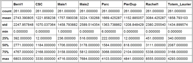
We can get some summary statistics of the table with the describe() method:
```
In [5]: df.describe()
```
Summary statistics of the DataFrame
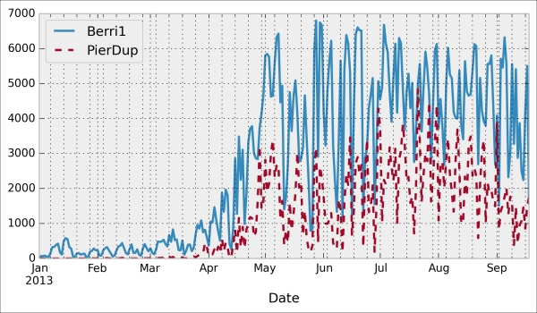
Let's display some figures. We will plot the daily attendance of two tracks. First, we select the two columns, Berri1 and PierDup. Then, we call the plot() method:
```
In [6]: df[['Berri1', 'PierDup']].plot()
```
Now, we move to a slightly more advanced analysis. We will look at the attendance of all tracks as a function of the weekday. We can get the weekday easily with pandas: the index attribute of the DataFrame object contains the dates of all rows in the table. This index has a few date-related attributes, including weekday:
```
In [7]: df.index.weekday
Out[7]: array([1, 2, 3, 4, 5, 6, 0, 1, 2, ..., 0, 1, 2])
```
However, we would like to have names (Monday, Tuesday, and so on) instead of numbers between 0 and 6. This can be done easily. First, we create a days array with all the weekday names. Then, we index it by df.index.weekday. This operation replaces every integer in the index by the corresponding name in days. The first element, Monday, has the index 0, so every 0 in df.index.weekday is replaced by Monday and so on. We assign this new index to a new column, Weekday, in DataFrame:
```
In [8]: days = np.array(['Monday', 'Tuesday', 'Wednesday', 
                         'Thursday', 'Friday', 'Saturday', 
                         'Sunday'])
        df['Weekday'] = days[df.index.weekday]
```
To get the attendance as a function of the weekday, we need to group the table elements by the weekday. The groupby() method lets us do just that. Once grouped, we can sum all the rows in every group:
```
In [9]: df_week = df.groupby('Weekday').sum()
In [10]: df_week
```
Grouped data with pandas
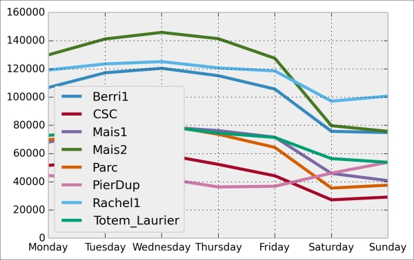
We can now display this information in a figure. We first need to reorder the table by the weekday using ix (indexing operation). Then, we plot the table, specifying the line width:
```
In [11]: df_week.ix[days].plot(lw=3)
         plt.ylim(0);  # Set the bottom axis to 0.
```
Finally, let's illustrate the new interactive capabilities of the notebook in IPython 2.0. We will plot a smoothed version of the track attendance as a function of time (rolling mean). The idea is to compute the mean value in the neighborhood of any day. The larger the neighborhood, the smoother the curve. We will create an interactive slider in the notebook to vary this parameter in real time in the plot. 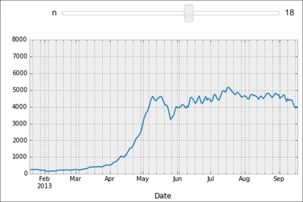All we have to do is add the @interact decorator above our plotting function:
```
In [12]: from IPython.html.widgets import interact
         @interact
         def plot(n=(1, 30)):
             pd.rolling_mean(df['Berri1'], n).dropna().plot()
             plt.ylim(0, 8000)
             plt.show()
```
Interactive widget in the notebook

There's more...

pandas is the right tool to load and manipulate a dataset. Other tools and methods are generally required for more advanced analyses (signal processing, statistics, and mathematical modeling). We will cover these steps in the second part of this book, starting with Chapter 7, Statistical Data Analysis.

Here are some more references about data manipulation with pandas:

Learning IPython for Interactive Computing and Data Visualization, Packt Publishing, our previous book
Python for Data Analysis, O'Reilly Media, by Wes McKinney, the creator of pandas
The documentation of pandas available at http://pandas.pydata.org/pandas-docs/stable/

IPython Interactive Computing and Visualization Cookbook

By : Cyrille Rossant

IPython Interactive Computing and Visualization Cookbook

By: Cyrille Rossant

Overview of this book

Getting started with exploratory data analysis in IPython

How to do it...

There's more...

See also

IPython Interactive Computing and Visualization Cookbook

By : Cyrille Rossant

IPython Interactive Computing and Visualization Cookbook

By: Cyrille Rossant

Overview of this book

Getting started with exploratory data analysis in IPython

How to do it...

There's more...

See also

Confirmation

Buy this book with your credits?

Submit Your Feedback

Create a Free Account To Continue Reading

Sign in to activate your 7-day free access