-
Book Overview & Buying

-
Table Of Contents

The Regularization Cookbook
By :
The Regularization Cookbook
By:
Overview of this book
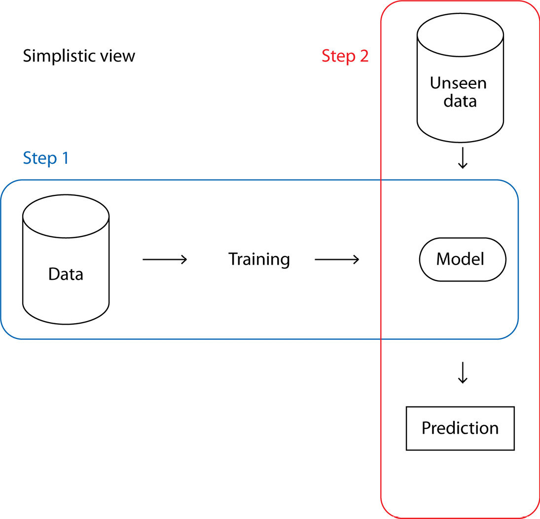
Regularization is an infallible way to produce accurate results with unseen data, however, applying regularization is challenging as it is available in multiple forms and applying the appropriate technique to every model is a must. The Regularization Cookbook provides you with the appropriate tools and methods to handle any case, with ready-to-use working codes as well as theoretical explanations.
After an introduction to regularization and methods to diagnose when to use it, you’ll start implementing regularization techniques on linear models, such as linear and logistic regression, and tree-based models, such as random forest and gradient boosting. You’ll then be introduced to specific regularization methods based on data, high cardinality features, and imbalanced datasets. In the last five chapters, you’ll discover regularization for deep learning models. After reviewing general methods that apply to any type of neural network, you’ll dive into more NLP-specific methods for RNNs and transformers, as well as using BERT or GPT-3. By the end, you’ll explore regularization for computer vision, covering CNN specifics, along with the use of generative models such as stable diffusion and Dall-E.
By the end of this book, you’ll be armed with different regularization techniques to apply to your ML and DL models.
Table of Contents (14 chapters)
Preface

Chapter 1: An Overview of Regularization
 Free Chapter
Chapter 2: Machine Learning Refresher
Chapter 3: Regularization with Linear Models
Chapter 4: Regularization with Tree-Based Models
Chapter 5: Regularization with Data
Chapter 6: Deep Learning Reminders
Chapter 7: Deep Learning Regularization
Chapter 8: Regularization with Recurrent Neural Networks
Chapter 9: Advanced Regularization in Natural Language Processing
Chapter 10: Regularization in Computer Vision
Chapter 11: Regularization in Computer Vision – Synthetic Image Generation
Index