Loading the Case Study Data with Jupyter and pandas
Now it's time to take a first look at the data we will use in our case study. We won't do anything in this section other than ensure that we can load the data into a Jupyter Notebook correctly. Examining the data, and understanding the problem you will solve with it, will come later.
The data file is an Excel spreadsheet called default_of_credit_card_clients__courseware_version_1_13_19.xls. We recommend you first open the spreadsheet in Excel, or the spreadsheet program of your choice. Note the number of rows and columns, and look at some example values. This will help you know whether or not you have loaded it correctly in the Jupyter Notebook.
Note
The dataset can obtained from the following link: http://bit.ly/2HIk5t3. This is a modified version of the original dataset, which has been sourced from the UCI Machine Learning Repository [http://archive.ics.uci.edu/ml]. Irvine, CA: University of California, School of Information and Computer Science.
What is a Jupyter Notebook?
Jupyter Notebooks are interactive coding environments that allow for in-line text and graphics. They are great tools for data scientists to communicate and preserve their results, since both the methods (code) and the message (text and graphics) are integrated. You can think of the environment as a kind of webpage where you can write and execute code. Jupyter Notebooks can, in fact, be rendered as web pages and are done so on GitHub. Here is one of our example notebooks: http://bit.ly/2OvndJg. Look it over and get a sense of what you can do. An excerpt from this notebook is displayed here, showing code, graphics, and prose, known as markdown in this context:
One of the first things to learn about Jupyter Notebooks is how to navigate around and make edits. There are two modes available to you. If you select a cell and press Enter, you are in edit mode and you can edit the text in that cell. If you press Esc, you are in command mode and you can navigate around the notebook.
When you are in command mode, there are many useful hotkeys you can use. The Up and Down arrows will help you select different cells and scroll through the notebook. If you press y on a selected cell in command mode, it changes it to a code cell, in which the text is interpreted as code. Pressing m changes it to a markdown cell. Shift + Enter evaluates the cell, rendering the markdown or executing the code, as the case may be.
Our first task in our first Jupyter Notebook will be to load the case study data. To do this, we will use a tool called pandas. It is probably not a stretch to say that pandas is the pre-eminent data-wrangling tool in Python.
A DataFrame is a foundational class in pandas. We'll talk more about what a class is later, but you can think of it as a template for a data structure, where a data structure is something like the lists or dictionaries we discussed earlier. However, a DataFrame is much richer in functionality than either of these. A DataFrame is similar to spreadsheets in many ways. There are rows, which are labeled by a row index, and columns, which are usually given column header-like labels that can be thought of as a column index. Index is, in fact, a data type in pandas used to store indices for a DataFrame, and columns have their own data type called Series.
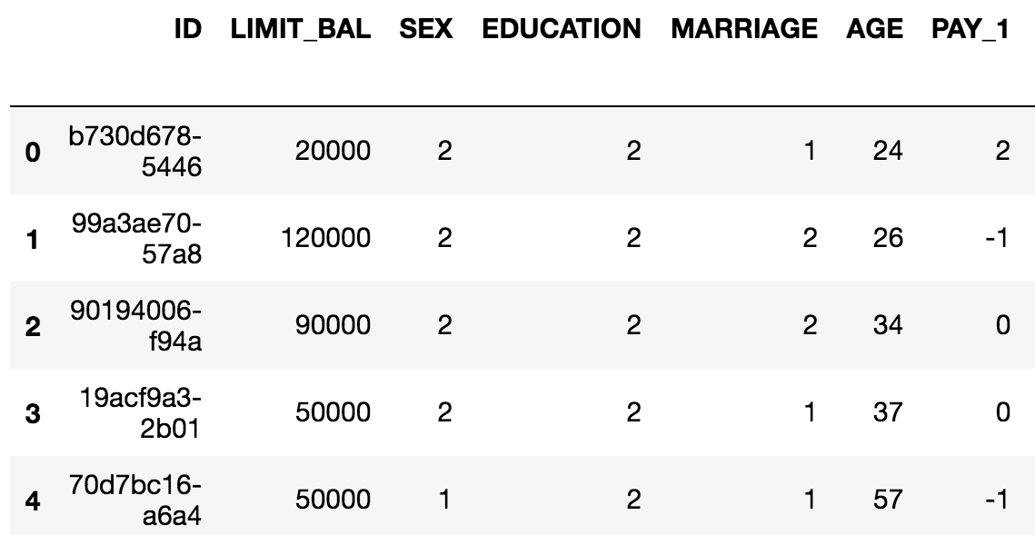
You can do a lot of the same things with a DataFrame that you can do with Excel sheets, such as creating pivot tables and filtering rows. pandas also includes SQL-like functionality. You can join different DataFrames together, for example. Another advantage of DataFrames is that once your data is contained in one of them, you have the capabilities of a wealth of pandas functionality at your fingertips. The following figure is an example of a pandas DataFrame:
The example in Figure 1.12 is in fact the data for the case study. As a first step with Jupyter and pandas, we will now see how to create a Jupyter Notebook and load data with pandas. There are several convenient functions you can use in pandas to explore your data, including .head() to see the first few rows of the DataFrame, .info() to see all columns with datatypes, .columns to return a list of column names as strings, and others we will learn about in the following exercises.
Exercise 2: Loading the Case Study Data in a Jupyter Notebook
Now that you've learned about Jupyter Notebooks, the environment in which we'll write code, and pandas, the data wrangling package, let's create our first Jupyter Notebook. We'll use pandas within this notebook to load the case study data and briefly examine it. Perform the following steps to complete the exercise:
Note
For Exercises 2–5 and Activity 1, the code and the resulting output have been loaded in a Jupyter Notebook that can be found at http://bit.ly/2W9cwPH. You can scroll to the appropriate section within the Jupyter Notebook to locate the exercise or activity of choice.
Open a Terminal (macOS or Linux) or a Command Prompt window (Windows) and type jupyter notebook.
You will be presented with the Jupyter interface in your web browser. If the browser does not open automatically, copy and paste the URL from the terminal in to your browser. In this interface, you can navigate around your directories starting from the directory you were in when you launched the notebook server.
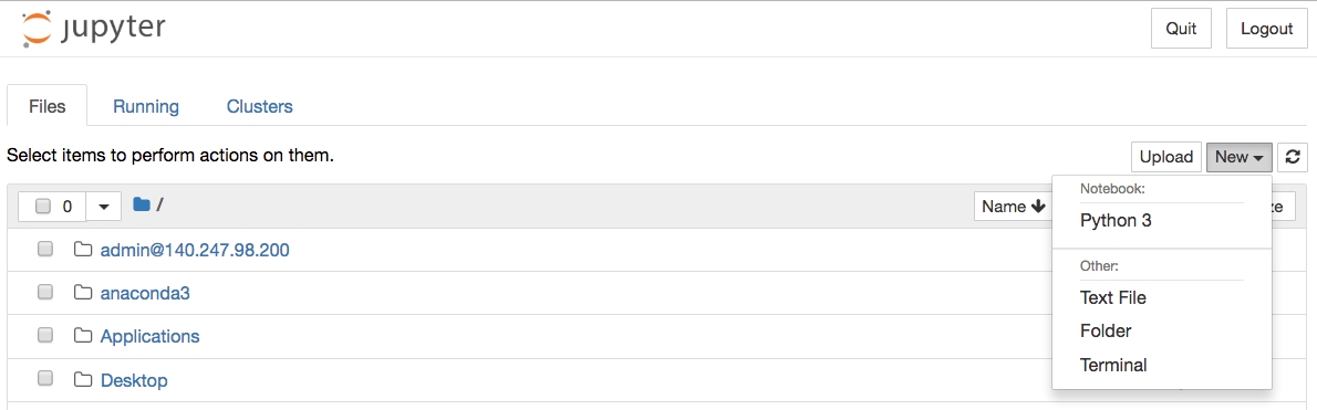
Navigate to a convenient location where you will store the materials for this book, and create a new Python 3 notebook from the New menu, as shown here:
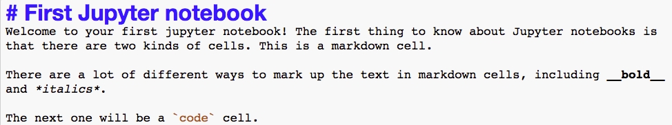
Make your very first cell a markdown cell by typing m while in command mode (press Esc to enter command mode), then type a number sign, #, at the beginning of the first line, followed by a space, for a heading. Make a title for your notebook here. On the next few lines, place a description.
Here is a screenshot of an example, including other kinds of markdown such as bold, italics, and the way to write code-style text in a markdown cell:
Note that it is good practice to make a title and brief description of your notebook, to identify its purpose to readers.
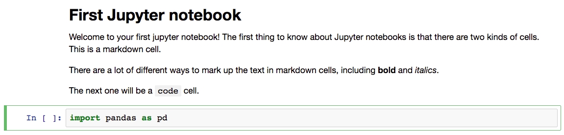
Press Shift + Enter to render the markdown cell.
This should also create a new cell, which will be a code cell. You can change it to a markdown cell, as you now know how to do, by pressing m, and back to a code cell by pressing y. You will know it's a code cell because of the In [ ]: next to it.
Type import pandas as pd in the new cell, as shown in the following screenshot:
After you execute this cell, the pandas library will be loaded into your computing environment. It's common to import libraries with "as" to create a short alias for the library. Now, we are going to use pandas to load the data file. It's in Microsoft Excel format, so we can use pd.read_excel.
Import the dataset, which is in the Excel format, as a DataFrame using the pd.read_excel() method, as shown in the following snippet:
Note that you need to point the Excel reader to wherever the file is located. If it's in the same directory as your notebook, you could just enter the filename. The pd.read_excel method will load the Excel file into a DataFrame, which we've called df. The power of pandas is now available to us.
Let's do some quick checks in the next few steps. First, do the numbers of rows and columns match what we know from looking at the file in Excel?
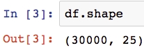
Use the .shape method to review the number of rows and columns, as shown in the following snippet:
Once you run the cell, you will obtain the following output:
This should match your observations from the spreadsheet. If it doesn't, you would then need to look into the various options of pd.read_excel to see if you needed to adjust something.
With this exercise, we have successfully loaded our dataset into the Jupyter Notebook. You can also have a look at the .info() and .head() methods, which will tell you information about all the columns, and show you the first few rows of the DataFrame, respectively. Now you're up and running with your data in pandas.
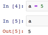
As a final note, while this may already be clear, observe that if you define a variable in one code cell, it is available to you in other code cells within the notebook. The code cells within a notebook share scope as long as the kernel is running, as shown in the following screenshot:
Getting Familiar with Data and Performing Data Cleaning
Now let's imagine we are taking our first look at this data. In your work as a data scientist, there are several possible scenarios in which you may receive such a dataset. These include the following:
You created the SQL query that generated the data.
A colleague wrote a SQL query for you, with your input.
A colleague who knows about the data gave it to you, but without your input.
You are given a dataset about which little is known.
In cases 1 and 2, your input was involved in generating/extracting the data. In these scenarios, you probably understood the business problem and then either found the data you needed with the help of a data engineer, or did your own research and designed the SQL query that generated the data. Often, especially as you gain more experience in your data science role, the first step will be to meet with the business partner to understand, and refine the mathematical definition of, the business problem. Then, you would play a key role in defining what is in the dataset.
Even if you have a relatively high level of familiarity with the data, doing data exploration and looking at summary statistics of different variables is still an important first step. This step will help you select good features, or give you ideas about how you can engineer new features. However, in the third and fourth cases, where your input was not involved or you have little knowledge about the data, data exploration is even more important.
Another important initial step in the data science process is examining the data dictionary. The data dictionary, as the term implies, is a document that explains what the data owner thinks should be in the data, such as definitions of the column labels. It is the data scientist's job to go through the data carefully to make sure that these impressions match the reality of what is in the data. In cases 1 and 2, you will probably need to create the data dictionary yourself, which should be considered essential project documentation. In cases 3 and 4, you should seek out the dictionary if at all possible.
The case study data we'll use in this book is basically similar to case 3 here.
Our client is a credit card company. They have brought us a dataset that includes some demographics and recent financial data (the past six months) for a sample of 30,000 of their account holders. This data is at the credit account level; in other words, there is one row for each account (you should always clarify what the definition of a row is, in a dataset). Rows are labeled by whether in the next month after the six month historical data period, an account owner has defaulted, or in other words, failed to make the minimum payment.
Goal
Your goal is to develop a predictive model for whether an account will default next month, given demographics and historical data. Later in the book, we'll discuss the practical application of the model.
The data is already prepared, and a data dictionary is available. The dataset supplied with the book, default_of_credit_card_clients__courseware_version_1_21_19.xls, is a modified version of this dataset in the UCI Machine Learning Repository: https://archive.ics.uci.edu/ml/datasets/default+of+credit+card+clients. Have a look at that web page, which includes the data dictionary.
Note
The original dataset has been obtained from UCI Machine Learning Repository [http://archive.ics.uci.edu/ml]. Irvine, CA: University of California, School of Information and Computer Science. In this book, we have modified the dataset to suit the book objectives. The modified dataset can be found here: http://bit.ly/2HIk5t3.
Now that we've understood the business problem and have an idea of what is supposed to be in the data, we can compare these impressions to what we actually see in the data. Your job in data exploration is to not only look through the data both directly and using numerical and graphical summaries, but also to think critically about whether the data make sense and match what you have been told about them. These are helpful steps in data exploration:
How many columns are there in the data?
These may be features, response, or metadata.
How many rows (samples)?
What kind of features are there? Which are categorical and which are numerical?
Categorical features have values in discrete classes such as "Yes," "No," or "maybe."Numerical features are typically on a continuous numerical scale, such as dollar amounts.
What does the data look like in these features?
To see this, you can examine the range of values in numeric features, or the frequency of different classes in categorical features, for example.
Is there any missing data?
We have already answered questions 1 and 2 in the previous section; there are 30,000 rows and 25 columns. As we start to explore the rest of these questions in the following exercise, pandas will be our go-to tool. We begin by verifying basic data integrity in the next exercise.
Note
Note that compared to the website's description of the data dictionary, X6-X11 are called PAY_1-PAY_6 in our data. Similarly, X12-X17 are BILL_AMT1-BILL_AMT6, and X18-X23 are PAY_AMT1-PAY_AMT6.
Exercise 3: Verifying Basic Data Integrity
In this exercise, we will perform a basic check on whether our dataset contains what we expect and verify whether there are the correct number of samples.
The data are supposed to have observations for 30,000 credit accounts. While there are 30,000 rows, we should also check whether there are 30,000 unique account IDs. It's possible that, if the SQL query used to generate the data was run on an unfamiliar schema, values that are supposed to be unique are in fact not unique.
To examine this, we can check if the number of unique account IDs is the same as the number of rows. Perform the following steps to complete the exercise:
Note
The code and the resulting output graphics for this exercise have been loaded in a Jupyter Notebook that can be found here: http://bit.ly/2W9cwPH.
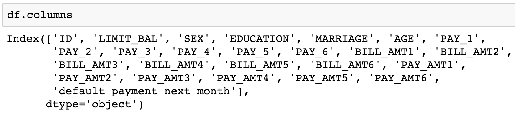
Examine the column names by running the following command in the cell:
The .columns method of the DataFrame is employed to examine all the column names. You will obtain the following output once you run the cell:
As can be observed, all column names are listed in the output. The account ID column is referenced as ID. The remaining columns appear to be our features, with the last column being the response variable. Let's quickly review the dataset information that was given to us by the client:
LIMIT_BAL: Amount of the credit provided (in New Taiwanese (NT) dollar) including individual consumer credit and the family (supplementary) credit.
SEX: Gender (1 = male; 2 = female).
Note
We will not be using the gender data to decide credit-worthiness owing to ethical considerations.
EDUCATION: Education (1 = graduate school; 2 = university; 3 = high school; 4 = others).
MARRIAGE: Marital status (1 = married; 2 = single; 3 = others).
AGE: Age (year).
PAY_1–Pay_6: A record of past payments. Past monthly payments, recorded from April to September, are stored in these columns.
PAY_1 represents the repayment status in September; PAY_2 = repayment status in August; and so on up to PAY_6, which represents the repayment status in April.
The measurement scale for the repayment status is as follows: -1 = pay duly; 1 = payment delay for one month; 2 = payment delay for two months; and so on up to 8 = payment delay for eight months; 9 = payment delay for nine months and above.
BILL_AMT1–BILL_AMT6: Bill statement amount (in NT dollar).
BILL_AMT1 represents the bill statement amount in September; BILL_AMT2 represents the bill statement amount in August; and so on up to BILL_AMT7, which represents the bill statement amount in April.
PAY_AMT1–PAY_AMT6: Amount of previous payment (NT dollar). PAY_AMT1 represents the amount paid in September; PAY_AMT2 represents the amount paid in August; and so on up to PAY_AMT6, which represents the amount paid in April.
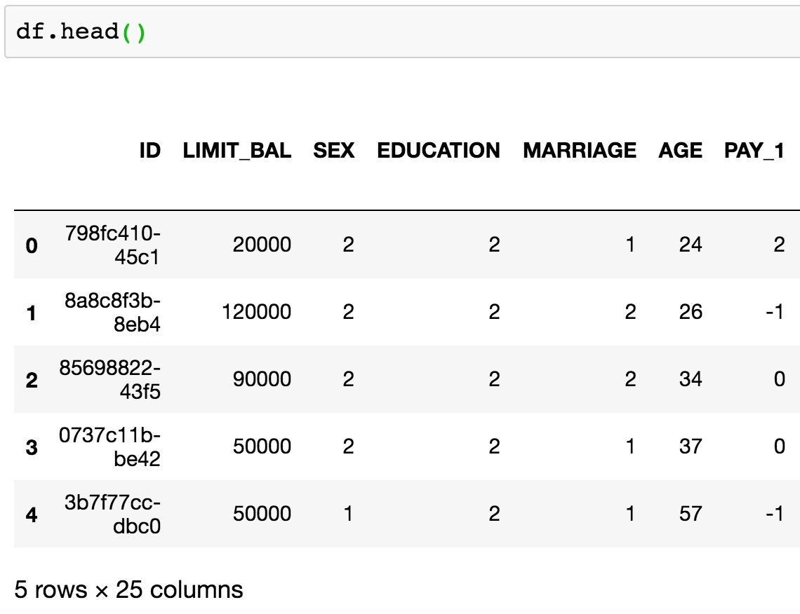
Let's now use the .head() method in the next step to observe the first few rows of data.
Type the following command in the subsequent cell and run it using Shift + Enter:
You will observe the following output:
The ID column seems like it contains unique identifiers. Now, to verify if they are in fact unique throughout the whole dataset, we can count the number of unique values using the .nunique() method on the Series (aka column) ID. We first select the column using square brackets.
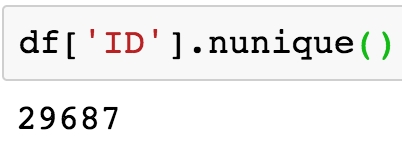
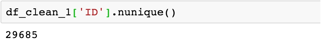
Select the target column (ID) and count unique values using the following command:
You will see in the following output that the number of unique entries is 29,687:
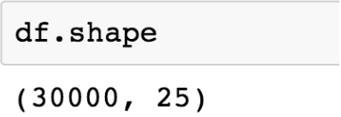
Run the following command to obtain the number of rows in the dataset:
As can be observed in the following output, the total number of rows in the dataset is 30,000:
We see here that the number of unique IDs is less than the number of rows. This implies that the ID is not a unique identifier for the rows of the data, as we thought. So we know that there is some duplication of IDs. But how much? Is one ID duplicated many times? How many IDs are duplicated?
We can use the .value_counts() method on the ID series to start to answer these questions. This is similar to a group by/count procedure in SQL. It will list the unique IDs and how often they occur. We will perform this operation in the next step and store the value counts in a variable id_counts.
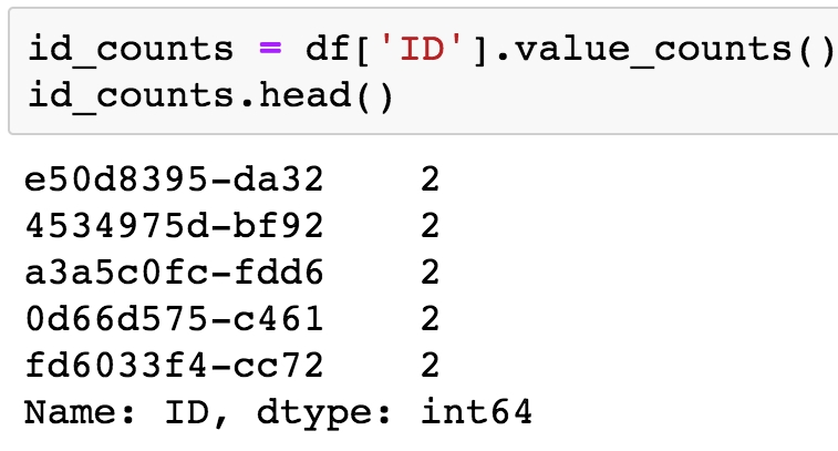
Store the value counts in a variable defined as id_counts and then display the stored values using the .head() method, as shown:
You will obtain the following output:
Note that .head() returns the first five rows by default. You can specify the number of items to be displayed by passing the required number in the parentheses, ().
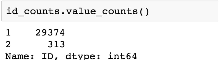
Display the number of grouped duplicated entries by running another value count:
You will obtain the following output:
In the preceding output and from the initial value count, we can see that most IDs occur exactly once, as expected. However, 313 IDs occur twice. So, no ID occurs more than twice. Armed with this information, we are ready to begin taking a closer look at this data quality issue and fixing it. We will be creating Boolean masks to further clean the data.
To help clean the case study data, we introduce the concept of a logical mask, also known as a Boolean mask. A logical mask is a way to filter an array, or series, by some condition. For example, we can use the "is equal to" operator in Python, ==, to find all locations of an array that contain a certain value. Other comparisons, such as "greater than" (>), "less than" (<), "greater than or equal to" (>=), and "less than or equal to" (<=), can be used similarly. The output of such a comparison is an array or series of True/False values, also known as Boolean values. Each element of the output corresponds to an element of the input, is True if the condition is met, and is False otherwise. To illustrate how this works, we will use synthetic data. Synthetic data is data that is created to explore or illustrate a concept. First, we are going to import the NumPy package, which has many capabilities for generating random numbers, and give it the alias np:
Now we use what's called a seed for the random number generator. If you set the seed, you will get the same results from the random number generator across runs. Otherwise this is not guaranteed. This can be a helpful option if you use random numbers in some way in your work and want to have consistent results every time you run a notebook:
Next, we generate 100 random integers, chosen from between 1 and 5 (inclusive). For this we can use numpy.random.randint, with the appropriate arguments.
Let's look at the first five elements of this array, with random_integers[:5]. The output should appear as follows:
Suppose we wanted to know the locations of all elements of random_integers equal to 3. We could create a Boolean mask to do this.
From examining the first 5 elements, we know the first element is equal to 3, but none of the rest are. So in our Boolean mask, we expect True in the first position and False in the next 4 positions. Is this the case?
The preceding code should give this output:
This is what we expected. This shows the creation of a Boolean mask. But what else can we do with them? Suppose we wanted to know how many elements were equal to 3. To know this, you can take the sum of a Boolean mask, which interprets True as 1 and False as 0:
This should give us the following output:
This makes sense, as with a random, equally likely choice of 5 possible values, we would expect each value to appear about 20% of the time. In addition to seeing how many values in the array meet the Boolean condition, we can also use the Boolean mask to select the elements of the original array that meet that condition. Boolean masks can be used directly to index arrays, as shown here:
This outputs the elements of random_integers meeting the Boolean condition we specified. In this case, the 22 elements equal to 3:
Now you know the basics of Boolean arrays, which are useful in many situations. In particular, you can use the .loc method of DataFrames to index the rows of the DataFrames by a Boolean mask, and the columns by label. Let's continue exploring the case study data with these skills.
Exercise 4: Continuing Verification of Data Integrity
In this exercise, with our knowledge of Boolean arrays, we will examine some of the duplicate IDs we discovered. In Exercise 3, we learned that no ID appears more than twice. We can use this learning to locate the duplicate IDs and examine them. Then we take action to remove rows of dubious quality from the dataset. Perform the following steps to complete the exercise:
Note
The code and the output graphics for this exercise have been loaded in a Jupyter Notebook that can be found here: http://bit.ly/2W9cwPH.
Continuing where we left off in Exercise 3, we want the indices of the id_counts series, where the count is 2, to locate the duplicates. We assign the indices of the duplicated IDs to a variable called dupe_mask and display the first 5 duplicated IDs using the following commands:
You will obtain the following output:
Here, dupe_mask is the logical mask that we have created for storing the Boolean values.
Note that in the preceding output, we are displaying only the first five entries using dupe_mask to illustrate to contents of this array. As always, you can edit the indices in the square brackets ([]) to change the number of entries displayed.
Our next step is to use this logical mask to select the IDs that are duplicated. The IDs themselves are contained as the index of the id_count series. We can access the index in order to use our logical mask for selection purposes.
Access the index of id_count and display the first five rows as context using the following command:
With this, you will obtain the following output:
Select and store the duplicated IDs in a new variable called dupe_ids using the following command:
Convert dupe_ids to a list and then obtain the length of the list using the following commands:
You should obtain the following output:
We changed the dupe_ids variable to a list, as we will need it in this form for future steps. The list has a length of 313, as can be seen in the preceding output, which matches our knowledge of the number of duplicate IDs from the value count.
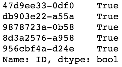
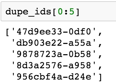
We verify the data in dupe_ids by displaying the first five entries using the following command:
We obtain the following output:
We can observe from the preceding output that the list contains the required entries of duplicate IDs. We're now in a position to examine the data for the IDs in our list of duplicates. In particular, we'd like to look at the values of the features, to see what, if anything, might be different between these duplicate entries. We will use the .isin and .loc methods for this purpose.
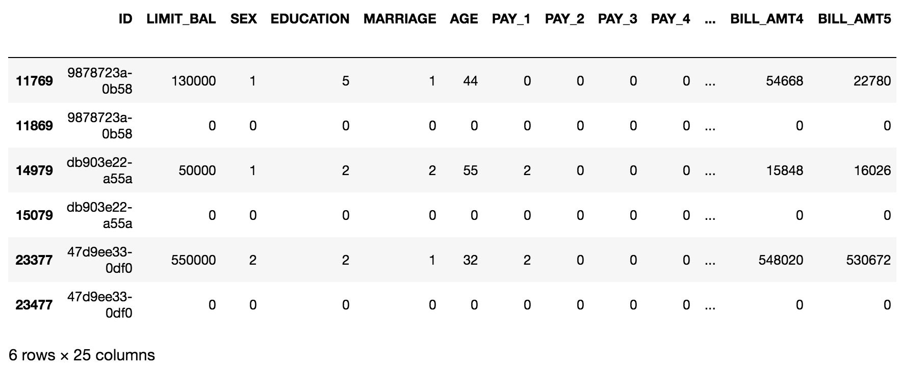
Using the first three IDs on our list of dupes, dupe_ids[0:3], we will plan to first find the rows containing these IDs. If we pass this list of IDs to the .isin method of the ID series, this will create another logical mask we can use on the larger DataFrame to display the rows that have these IDs. The .isin method is nested in a .loc statement indexing the DataFrame in order to select the location of all rows containing "True" in the Boolean mask. The second argument of the .loc indexing statement is :, which implies that all columns will be selected. By performing the following steps, we are essentially filtering the DataFrame in order to view all the columns for the first three duplicate IDs.
Run the following command in your Notebook to execute the plan we formulated in the previous step:
What we observe here is that each duplicate ID appears to have one row with what seems like valid data, and one row of entirely zeros. Take a moment and think to yourself what you would do with this knowledge.
After some reflection, it should be clear that you ought to delete the rows with all zeros. Perhaps these arose through a faulty join condition in the SQL query that generated the data? Regardless, a row of all zeros is definitely invalid data as it makes no sense for someone to have an age of 0, a credit limit of 0, and so on.
One approach to deal with this issue would be to find rows that have all zeros, except for the first column, which has the IDs. These would be invalid data in any case, and it may be that if we get rid of all of these, we would also solve our problem of duplicate IDs. We can find the entries of the DataFrame that are equal to zero by creating a Boolean matrix that is the same size as the whole DataFrame, based on the "is equal to zero" condition.
Create a Boolean matrix of the same size as the entire DataFrame using ==, as shown:
In the next steps, we'll use df_zero_mask, which is another DataFrame containing Boolean values. The goal will be to create a Boolean series, feature_zero_mask, that identifies every row where all the elements starting from the second column (the features and response, but not the IDs) are 0. To do so, we first need to index df_zero_mask using the integer indexing (.iloc) method. In this method, we pass (:) to examine all rows and (1:) to examine all columns starting with the second one (index 1). Finally, we will apply the all() method along the column axis (axis=1), which will return True if and only if every column in that row is True. This is a lot to think about, but it's pretty simple to code, as will be observed in the following step.
Create the Boolean series feature_zero_mask, as shown in the following:
Calculate the sum of the Boolean series using the following command:
You should obtain the following output:
The preceding output tells us that 315 rows have zeros for every column but the first one. This is greater than the number of duplicate IDs (313), so if we delete all the "zero rows," we may get rid of the duplicate ID problem.
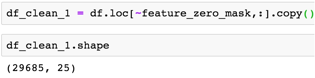
Clean the DataFrame by eliminating the rows with all zeros, except for the ID, using the following code:
While performing the cleaning operation in the preceding step, we return a new DataFrame called df_clean_1. Notice that here we've used the .copy() method after the .loc indexing operation to create a copy of this output, as opposed to a view on the original DataFrame. You can think of this as creating a new DataFrame, as opposed to referencing the original one. Within the .loc method, we used the logical not operator, ~, to select all the rows that don't have zeros for all the features and response, and : to select all columns. These are the valid data we wish to keep. After doing this, we now want to know if the number of remaining rows is equal to the number of unique IDs.
Verify the number of rows and columns in df_clean_1 by running the following code:
You will obtain the following output:
Obtain the number of unique IDs by running the following code:
From the preceding output, we can see that we have successfully eliminated duplicates, as the number of unique IDs is equal to the number of rows. Now take a breath and pat yourself on the back. That was a whirlwind introduction to quite a few pandas techniques for indexing and characterizing data. Now that we've filtered out the duplicate IDs, we're in a position to start looking at the actual data itself: the features, and eventually, the response. We'll walk you through this process.
Exercise 5: Exploring and Cleaning the Data
Thus far, we have identified a data quality issue related to the metadata: we had been told that every sample from our dataset corresponded to a unique account ID, but found that this was not the case. We were able to use logical indexing and pandas to correct this issue. This was a fundamental data quality issue, having to do simply with what samples were present, based on the metadata. Aside from this, we are not really interested in the metadata column of account IDs: for the time being these will not help us develop a predictive model for credit default.
Now, we are ready to start examining the values of the features and response, the data we will use to develop our predictive model. Perform the following steps to complete this exercise:
Note
The code and the resulting output for this exercise have been loaded in a Jupyter Notebook that can be found here: http://bit.ly/2W9cwPH.
-2 means the account started that month with a zero balance, and never used any credit
-1 means the account had a balance that was paid in full
0 means that at least the minimum payment was made, but the entire balance wasn't paid (that is, a positive balance was carried to the next month)
We thank our business partner since this answers our questions, for now. Maintaining a good line of communication and working relationship with the business partner is important, as you can see here, and may determine the success or failure of a project.
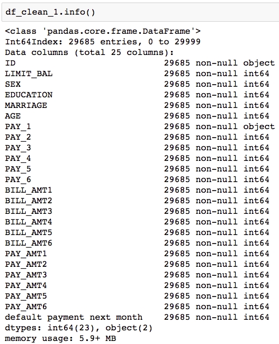
Obtain the data type of the columns in the data by using the .info() method as shown:
You should see the following output:
We can see in Figure 1.34 that there are 25 columns. Each row has 29,685 non-null values, according to this summary, which is the number of rows in the DataFrame. This would indicate that there is no missing data, in the sense that each cell contains some value. However, if there is a fill value to represent missing data, that would not be evident here.
We also see that most columns say int64 next to them, indicating they are an integer data type, that is, numbers such as ..., -2, -1, 0, 1, 2,... . The exceptions are ID and PAY_1. We are already familiar with ID; this contains strings, which are account IDs. What about PAY_1? According to the values in the data dictionary, we'd expect this to contain integers, like all the other features. Let's take a closer look at this column.
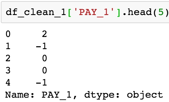
Use the.head(n) pandas method to view the top n rows of the PAY_1 series:
You should obtain the following output:
The integers on the left of the output are the index, which are simply consecutive integers starting with 0. The data from the PAY_1 column is shown on the left. This is supposed to be the payment status of the most recent month's bill, using values –1, 1, 2, 3, and so on. However, we can see that there are values of 0 here, which are not documented in the data dictionary. According to the data dictionary, "The measurement scale for the repayment status is: -1 = pay duly; 1 = payment delay for one month; 2 = payment delay for two months; . . .; 8 = payment delay for eight months; 9 = payment delay for nine months and above" (https://archive.ics.uci.edu/ml/datasets/default+of+credit+card+clients). Let's take a closer look, using the value counts of this column.
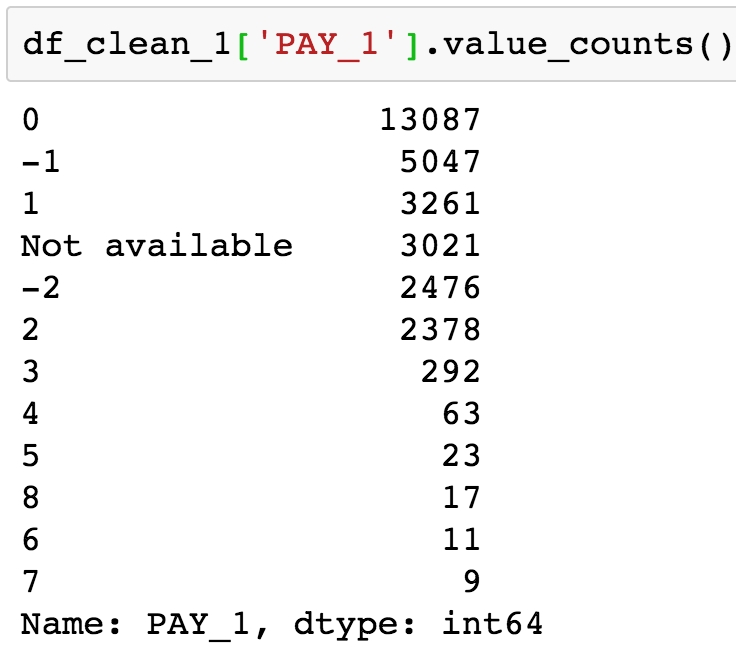
Obtain the value counts for the PAY_1 column by using .value_counts() method:
You should see the following output:
The preceding output reveals the presence of two undocumented values: 0 and –2, as well as the reason this column was imported by pandas as an object data type, instead of int64 as we would expect for integer data. There is a 'Not available' string present in this column, symbolizing missing data. Later on in the book, we'll come back to this when we consider how to deal with missing data. For now, we'll remove rows of the dataset, for which this feature has a missing value.
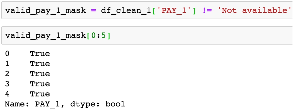
Use a logical mask with the != operator (which means "does not equal" in Python) to find all the rows that don't have missing data for the PAY_1 feature:
By running the preceding code, you will obtain the following output:
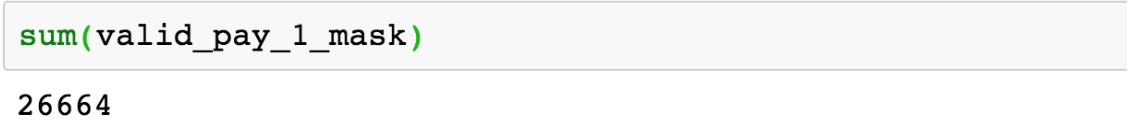
Check how many rows have no missing data by calculating the sum of the mask:
You will obtain the following output:
We see that 26,664 rows do not have the value 'Not available' in the PAY_1 column. We saw from the value count that 3,021 rows do have this value, and 29,685 – 3,021 = 26,664, so this checks out.
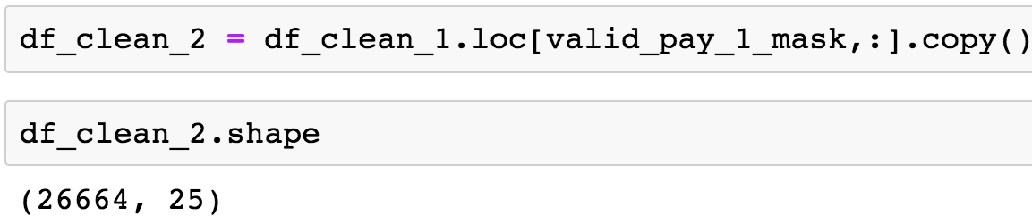
Clean the data by eliminating the rows with the missing values of PAY_1 as shown:
Obtain the shape of the cleaned data using the following command:
You will obtain the following output:
After removing these rows, we check that the resulting DataFrame has the expected shape. You can also check for yourself whether the value counts indicate the desired values have been removed like this: df_clean_2['PAY_1'].value_counts().
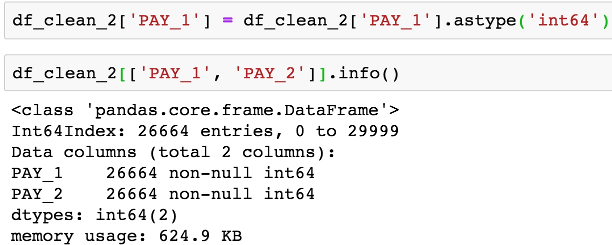
Lastly, so this column's data type can be consistent with the others, we will cast it from the generic object type to int64 like all the other features, using the .astype method. Then we select a couple columns, including PAY_1, to examine the data types and make sure it worked.
Run the following command to convert the data type for PAY_1 from object to int64 and show the column metadata for PAY_1 and PAY_2:
Congratulations, you have completed your second data cleaning operation! However, if you recall, during this process we also noticed the undocumented values of –2 and 0 in PAY_1. Now, let's imagine we got back in touch with our business partner and learned the following information:


 Free Chapter