Data Preparation

The first step in the development of any deep learning model – after gathering the data, of course – should be preparation of the data. This is crucial if we wish to understand the data at hand to outline the scope of the project correctly.

Many data scientists fail to do so, which results in models that perform poorly, and even models that are useless as they do not answer the data problem to begin with.

The process of preparing the data can be divided into three main tasks:

1. Understanding the data and dealing with any potential issues
2. Rescaling the features to make sure no bias is introduced by mistake
3. Splitting the data to be able to measure performance accurately

All three tasks will be further explained in the next section.

Note

All of the tasks we explained previously are pretty much the same when applying any machine learning algorithm, considering that they refer to the techniques that are required to prepare data beforehand.

Dealing with Messy Data

This task mainly consists of performing exploratory data analysis (EDA) to understand the data available, as well as to detect potential issues that may affect the development of the model.

The EDA process is useful as it helps the developer uncover information that's crucial to the definition of the course of action. This information is explained here:

1. Quantity of data: This refers both to the number of instances and the number of features. The former is crucial for determining whether it is necessary or even possible to solve the data problem using a neural network, or even a deep neural network, considering that such models require vast amounts of data to achieve high levels of accuracy. The latter, on the other hand, is useful for determining whether it would be a good practice to develop some feature selection methodologies beforehand in order to reduce the number of features, to simplify the model, and to eliminate any redundant information.
2. The target feature: For supervised models, data needs to be labeled. Considering this, it is highly important to select the target feature (the objective that we want to achieve by building the model) in order to assess whether the feature has many missing or outlier values. Additionally, this helps determine the objective of the development, which should be in line with the data that's available.
3. Noisy data/outliers: Noisy data refers to values that are visibly incorrect, for instance, a person who is 200 years old. On the other hand, outliers refer to values that, although they may be correct, are very far from the mean, for instance, a 10-year-old college student.

   There is not an exact science for detecting outliers, but there are some methodologies that are commonly accepted. Assuming a normally distributed dataset, one of the most popular ones is determining any value that is about 3-6 standard deviations away from the mean as an outlier.

   An equally valid approach to identifying outliers is to select those values at the 99th and 1st percentiles.

   It is very important to handle such values when they represent over 5% of the data for a feature because failing to do so may introduce bias to the model. The way to handle these values, as with any other machine learning algorithm, is to either delete the outlier values or assign new values using mean or regression imputation techniques.

4. Missing values: Similar to the aforementioned, a dataset with many missing values can introduce bias to the model, considering that different models will make different assumptions about those values. Again, when missing values represent over 5% of the values of a feature, they should be handled by eliminating or replacing them, again using the mean or regression imputation techniques.
5. Qualitative features: Finally, checking whether the dataset contains qualitative data is also a key step, considering that removing or encoding data may result in more accurate models.

   Additionally, in many research developments, several algorithms are tested on the same data in order to determine which one performs better, and some of these algorithms do not tolerate the use of qualitative data, as is the case with neural networks. This proves the importance of converting or encoding them to be able to feed all the algorithms the same data.

Exercise 2.02: Dealing with Messy Data

Note

All of the exercises in this chapter will be completed using the Appliances energy prediction Dataset sourced from the UC Irvine Machine Learning Repository, which was downloaded from https://archive.ics.uci.edu/ml/datasets/Appliances+energy+prediction. It can also be found in this book's GitHub repository: https://packt.live/34MBoSw

The Appliances energy prediction Dataset contains 4.5 months of data related to temperature and humidity measures for different rooms in a low-energy building, with the objective of predicting the energy that's used by certain appliances.

In this exercise, we will use pandas, which is a popular Python package, to explore the data at hand and learn how to detect missing values, outliers, and qualitative values. Perform the following steps to complete this exercise:

Note

For the exercises and activities within this chapter, you will need to have Python 3.7, Jupyter 6.0, NumPy 1.17, and Pandas 0.25 installed on your local machine.

1. Open a Jupyter notebook to implement this exercise.
2. Import the pandas library:

   import pandas as pd

3. Use pandas to read the CSV file containing the dataset we downloaded from the UC Irvine Machine Learning Repository site.

   Next, drop the column named date as we do not want to consider it for the following exercises:

   data = pd.read_csv("energydata_complete.csv")
   data = data.drop(columns=["date"])

   Finally, print the head of the DataFrame:

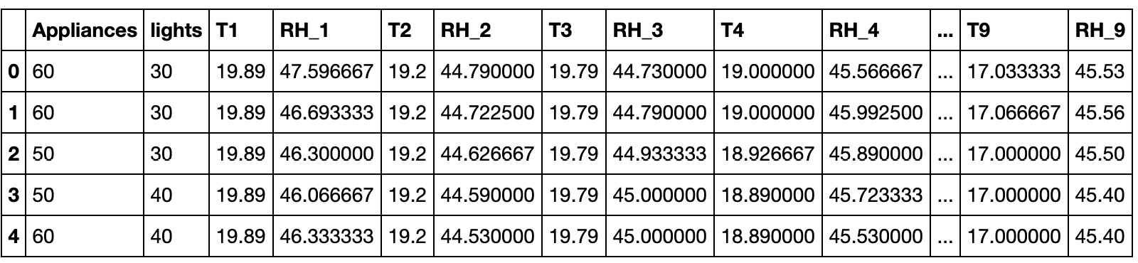
   data.head()

   The output should look as follows:

   

   Figure 2.26: Top instances of the Appliances energy prediction dataset

4. Check for categorical features in your dataset:

   cols = data.columns
   num_cols = data._get_numeric_data().columns
   list(set(cols) - set(num_cols))

   The first line generates a list of all the columns in your dataset. Next, the columns that contain numeric values are stored in a variable as well. Finally, by subtracting the numeric columns from the entire list of columns, it is possible to obtain those that are not numeric.

   The resulting list is empty, which indicates that there are no categorical features to deal with.

5. Use Python's isnull() and sum() functions to find out whether there are any missing values in each column of the dataset:

   data.isnull().sum()

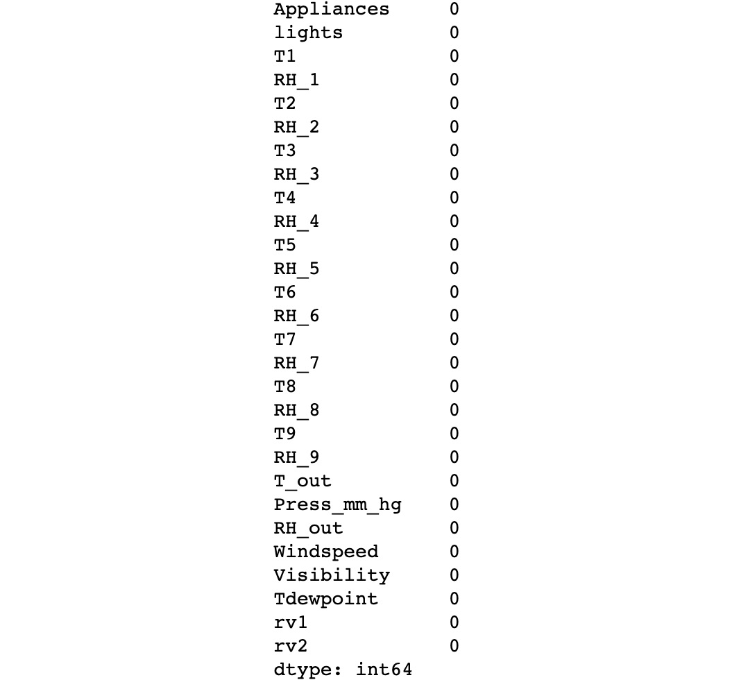
   This command counts the number of null values in each column. For the dataset in use, there should not be any missing values, as can be seen here:

   

   Figure 2.27: Missing values count

6. Use three standard deviations as the measure to detect any outliers for all the features in the dataset:

   outliers = {}
   for i in range(data.shape[1]):
       min_t = data[data.columns[i]].mean() \
               - (3 * data[data.columns[i]].std())
       max_t = data[data.columns[i]].mean() \
               + (3 * data[data.columns[i]].std())
       count = 0
       for j in data[data.columns[i]]:
           if j < min_t or j > max_t:
               count += 1
       percentage = count / data.shape[0]
       outliers[data.columns[i]] = "%.3f" % percentage
   outliers

   The preceding code snippet performs a for loop through the columns in the dataset in order to evaluate the presence of outliers in each of them. It continues to calculate the minimum and maximum thresholds so that it can count the number of instances that fall outside the range between the thresholds.

   Finally, it calculates the percentage of outliers (that is, the number of outliers divided by the total number of instances) in order to output a dictionary that displays this percentage for each column.

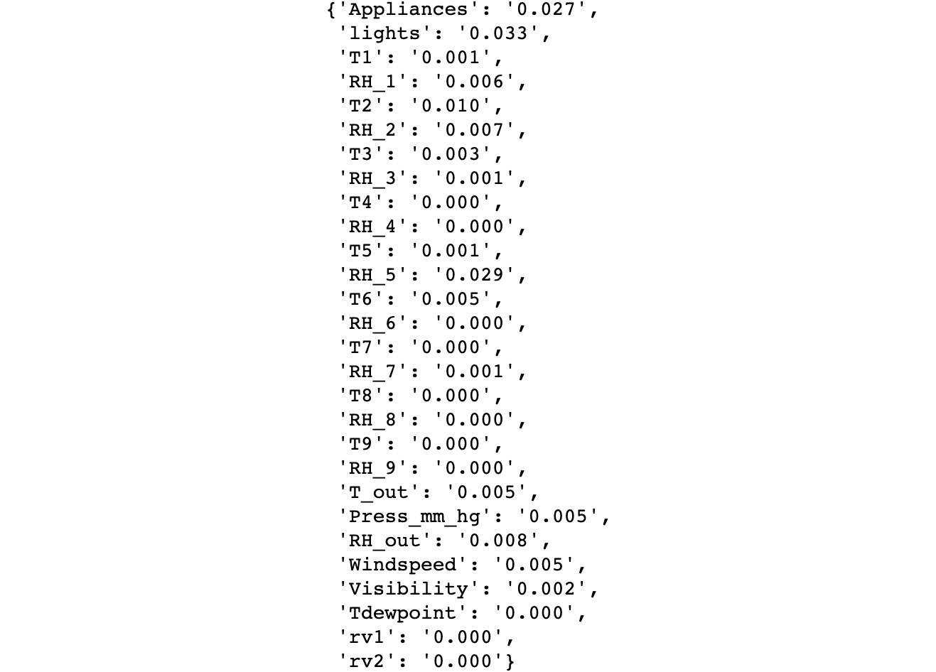
   By printing the resulting dictionary (outliers), it is possible to display a list of all the features (columns) in the dataset, along with the percentage of outliers. According to the result, it is possible to conclude that there is no need to deal with the outlier values, considering that they account for less than 5% of the data, as can be seen in the following screenshot:

   Note

   Note that Jupyter Notebooks can print the value of a variable without the need for the print function whenever the variable is placed at the end of a cell in the notebook. In any other programming platform or any other scenario, make sure to use the print function.

   For instance, an equivalent way (and the best practice) to print the resulting dictionary containing the outliers would be to use the print statement, as follows: print(outliers). This way, the code will have the same output when run in a different programming platform.

Figure 2.28: Outlier participation in each feature

Note

To access the source code for this specific section, please refer to https://packt.live/2CYEglp.

You can also run this example online at https://packt.live/3ePAg4G. You must execute the entire Notebook in order to get the desired result.

You have successfully explored the dataset and dealt with potential issues.

Data Rescaling

Although data does not need to be rescaled to be fed to an algorithm for training, it is an important step if you wish to improve a model's accuracy. This is basically because having different scales for each feature may result in the model assuming that a given feature is more important than others as it has higher numerical values.

Take, for instance, two features, one measuring the number of children a person has and another stating the age of the person. Even though the age feature may have higher numerical values, in a study for recommending schools, the number of children feature may be more important.

Considering this, if all the features are scaled equally, the model can actually give higher weights to those features that matter the most in respect to the target feature, and not the numerical values that they have. Moreover, it can also help accelerate the training process by removing the need for the model to learn from the invariance of the data.

There are two main rescaling methodologies that are popular among data scientists, and although there is no rule for selecting one or the other, it is important to highlight that they are to be used individually (one or the other).

A brief explanation of both of these methodologies can be found here:

• Normalization: This consists of rescaling the values so that all the values of all the features are between zero and one. This is done using the following equation:

Figure 2.29: Data normalization

• Standardization: In contrast, this rescaling methodology converts all the values so that their mean is 0 and their standard deviation is equal to 1. This is done using the following equation:

Figure 2.30: Data standardization

Exercise 2.03: Rescaling Data

In this exercise, we will rescale the data from the previous exercise. Perform the following steps to do so:

Note

Use the same Jupyter notebook that you used in the previous exercise.

1. Separate the features from the target. We are only doing this to rescale the features data:

   X = data.iloc[:, 1:]
   Y = data.iloc[:, 0]

   The preceding code snippet takes the data and uses slicing to separate the features from the target.

2. Rescale the features data by using the normalization methodology. Display the head (that is, the top five instances) of the resulting DataFrame to verify the result:

   X = (X - X.min()) / (X.max() - X.min())
   X.head()

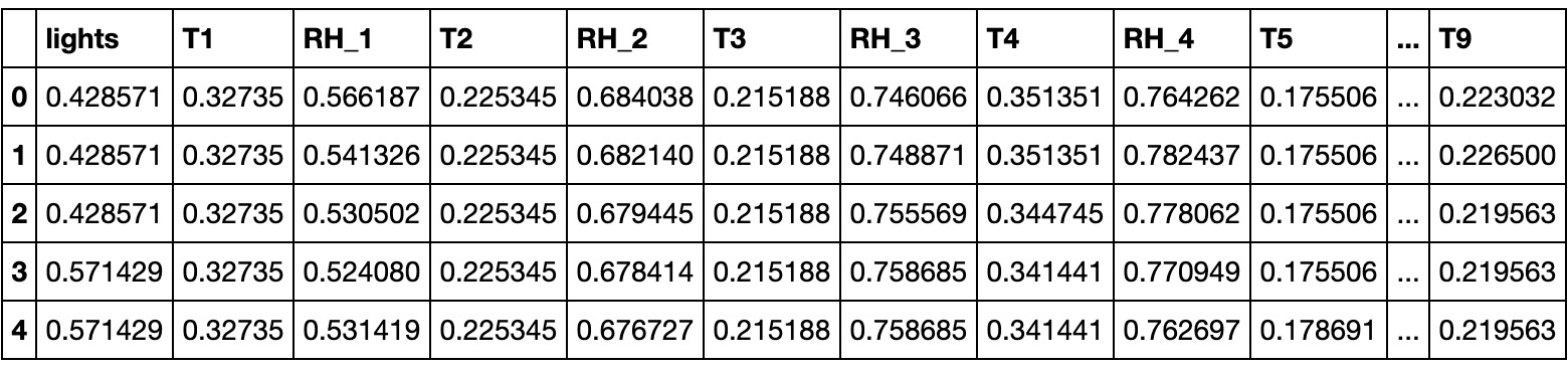
   The output should look as follows:

Figure 2.31: Top instances of the normalized Appliances energy prediction dataset

Note

To access the source code for this specific section, please refer to https://packt.live/2ZojumJ.

You can also run this example online at https://packt.live/2NLVgxq. You must execute the entire Notebook in order to get the desired result.

You have successfully rescaled a dataset.

Splitting the Data

The purpose of splitting the dataset into three subsets is so that the model can be trained, fine-tuned, and measured appropriately, without the introduction of bias. Here is an explanation of each set:

• Training set: As its name suggests, this set is fed to the neural network to be trained. For supervised learning, it consists of the features and the target values. This is typically the largest set out of the three, considering that neural networks require large amounts of data to be trained, as we mentioned previously.
• Validation set (dev set): This set is used mainly to measure the performance of the model in order to make adjustments to the hyperparameters to improve performance. This fine-tuning process is done so that we can configure the hyperparameters that achieve the best results.

  Although the model is not trained on this data, it indirectly has an effect on it, which is why the final measure of performance should not be done on it as it may be a biased measure.

• Testing set: This set does not have an effect on the model, which is why it is used to perform a final evaluation of the model on unseen data, which becomes a guideline of how well the model will perform on future datasets.

There is no actual science on the perfect ratio for splitting data into the three sets mentioned, considering that every data problem is different and developing deep learning solutions usually requires a trial-and-error methodology. Nevertheless, it is widely known that larger datasets (hundreds of thousands and millions of instances) should have a split ratio of 98:1:1 for each set, considering that it is crucial to use as much data as possible for the training set. For a smaller dataset, the conventional split ratio is 60:20:20.

Exercise 2.04: Splitting a Dataset

In this exercise, we will split the dataset from the previous exercise into three subsets. For the purpose of learning, we will explore two different approaches. First, the dataset will be split using indexing. Next, scikit-learn's train_test_split() function will be used for the same purpose, thereby achieving the same result with both approaches. Perform the following steps to complete this exercise:

Note

Use the same Jupyter notebook that you used in the previous exercise.

1. Print the shape of the dataset in order to determine the split ratio to be used:

   X.shape

   The output from this operation should be (19735, 27). This means that it is possible to use a split ratio of 60:20:20 for the training, validation, and test sets.

2. Get the value that you will use as the upper bound of the training and validation sets. This will be used to split the dataset using indexing:

   train_end = int(len(X) * 0.6)
   dev_end = int(len(X) * 0.8)

   The preceding code determines the index of the instances that will be used to divide the dataset through slicing.

3. Shuffle the dataset:

   X_shuffle = X.sample(frac=1, random_state=0)
   Y_shuffle = Y.sample(frac=1, random_state=0)

   Using the pandas sample function, it is possible to shuffle the elements in the features and target matrices. By setting frac to 1, we ensure that all the instances are shuffled and returned in the output from the function. Using the random_state argument, we ensure that both datasets are shuffled equally.

4. Use indexing to split the shuffled dataset into the three sets for both the features and the target data:

   x_train = X_shuffle.iloc[:train_end,:]
   y_train = Y_shuffle.iloc[:train_end]
   x_dev = X_shuffle.iloc[train_end:dev_end,:]
   y_dev = Y_shuffle.iloc[train_end:dev_end]
   x_test = X_shuffle.iloc[dev_end:,:]
   y_test = Y_shuffle.iloc[dev_end:]

5. Print the shapes of all three sets:

   print(x_train.shape, y_train.shape)
   print(x_dev.shape, y_dev.shape)
   print(x_test.shape, y_test.shape)

   The result of the preceding operation should be as follows:

   (11841, 27) (11841,)
   (3947, 27) (3947,)
   (3947, 27) (3947,)

6. Import the train_test_split() function from scikit-learn's model_selection module:

   from sklearn.model_selection import train_test_split

   Note

   Although the different packages and libraries are being imported as they are needed for practical learning purposes, it is always good practice to import them at the beginning of your code.

7. Split the shuffled dataset:

   x_new, x_test_2, \
   y_new, y_test_2 = train_test_split(X_shuffle, Y_shuffle, \
                                      test_size=0.2, \
                                      random_state=0)
   dev_per = x_test_2.shape[0]/x_new.shape[0]
   x_train_2, x_dev_2, \
   y_train_2, y_dev_2 = train_test_split(x_new, y_new, \
                                         test_size=dev_per, \
                                         random_state=0)

   The first line of code performs an initial split. The function takes the following as arguments:

   X_shuffle, Y_shuffle: The datasets to be split, that is, the features dataset, as well as the target dataset (also known as X and Y)

   test_size: The percentage of instances to be contained in the testing set

   random_state: Used to ensure the reproducibility of the results

   The result from this line of code is the division of each of the datasets (X and Y) into two subsets.

   To create an additional set (the validation set), we will perform a second split. The second line of the preceding code is in charge of determining the test_size to be used for the second split so that both the testing and validation sets have the same shape.

   Finally, the last line of code performs the second split using the value that was calculated previously as the test_size.

8. Print the shape of all three sets:

   print(x_train_2.shape, y_train_2.shape)
   print(x_dev_2.shape, y_dev_2.shape)
   print(x_test_2.shape, y_test_2.shape)

   The result from the preceding operation should be as follows:

   (11841, 27) (11841,)
   (3947, 27) (3947,)
   (3947, 27) (3947,)

   As we can see, the resulting sets from both approaches have the same shapes. Using one approach or the other is a matter of preference.

   Note

   To access the source code for this specific section, please refer to https://packt.live/2VxvroW.

   You can also run this example online at https://packt.live/3gcm5H8. You must execute the entire Notebook in order to get the desired result.

You have successfully split the dataset into three subsets.

Disadvantages of Failing to Prepare Your Data

Although the process of preparing the dataset is time-consuming and may be tiring when dealing with large datasets, the disadvantages of failing to do so are even more inconvenient:

• Longer training times: Data containing noise, missing values, and redundant or irrelevant columns takes considerably longer to train and, in most cases, this delay in time is even longer than the time it takes to prepare the data. For instance, during data preparation, it may be determined that five columns are irrelevant for the purpose of the study, which may reduce the dataset considerably, and hence reduce the training times considerably.
• Introduction of bias: Uncleaned data usually contains errors or missing values that can deviate the model from the truth. For instance, missing values can cause the model to make inferences that are not true, which, in turn, creates a model that does not represent the data.
• Avoid generalization: Outliers and noisy values prevent the model from making generalizations of the data, which is crucial for building a model that represents the current training data, as well as future unseen data. For example, a dataset containing a variable for age that contains entries of people who are over 100 years old may result in a model that accounts for those users who, in reality, represent a very small portion of the population.

Activity 2.01: Performing Data Preparation

In this activity, we will prepare a dataset containing a list of songs, each with several attributes that help determine the year they were released. This data preparation step is crucial for the next activity in this chapter. Let's look at the following scenario.

You work at a music record company and your boss wants to uncover the details that characterize records from different time periods, which is why they have put together a dataset that contains data on 515,345 records, with release years ranging from 1922 to 2011. They have tasked you with preparing the dataset so that it is ready to be fed to a neural network. Perform the following steps to complete this activity:

Note

To download the dataset for this activity, visit the following UC Irvine Machine Learning Repository URL: https://archive.ics.uci.edu/ml/datasets/YearPredictionMSD.

Citation: Dua, D. and Graff, C. (2019). UCI Machine Learning Repository [http://archive.ics.uci.edu/ml]. Irvine, CA: University of California, School of Information and Computer Science.

It is also available at this book's GitHub repository: https://packt.live/38kZzZR

1. Import the required libraries.
2. Using pandas, load the .csv file.
3. Verify whether any qualitative data is present in the dataset.
4. Check for missing values.

   You can also add an additional sum() function to get the sum of missing values in the entire dataset, without discriminating by column.

5. Check for outliers.
6. Separate the features from the target data.
7. Rescale the data using the standardization methodology.
8. Split the data into three sets: training, validation, and test. Use whichever approach you prefer.

   Note

   The solution for this activity can be found via this link.