
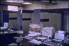
The descriptor super computing first appeared in the publication New York World in 1929. The term was in reference to the large, custom-built IBM tabulator installed at Columbia University. The IBM tabulator is depicted following:
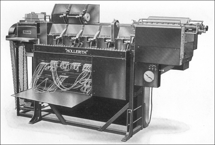
IBM Tabulators and Accounting Machine
The burgeoning supercomputing field was later buttressed with contributions from the famed Seymour Cray, with his brainchild, the CDC6600, that appeared in 1964. The machine, for all intents and purposes, was the first supercomputer. Cray was an applied mathematician, computer scientist, and electrical engineer. He subsequently built many faster machines. He passed away on October 5, 1996 (age 71) but his legacy lives on today in several powerful supercomputers bearing his name.
The quest for the exaflop machine (a billion, billion calculations per second) commenced when computer engineers in the 1980s gave birth to a slew of supercomputers that only had a few processors. In the 1990s, machines that had thousands of processors began appearing in the United States and Japan. These machines achieved new teraflop (1,000 billion calculations per second) processing performance records, but this achievement was only fleeting, as the end of the 20th century ushered in petaflop (1,000,000 billion calculations per second) machines that had large-scale parallel architecture. These machines comprise thousands (over 60,000, to give an estimate) of off-the-shelf processors similar to those used in personal computers. Indeed, progress in performance is relentless, and inexorable - maybe? I guess only time will tell. An image of an early trailblazing supercomputer, the Cray-1, is depicted in the following figure:
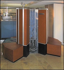
A Cray-1 supercomputer preserved at the Deutsches Museum
The relentless drive for ever-greater computing power began in earnest in 1957 when a splinter group of engineers left the Sperry Corporation to launched the Minneapolis, MN based Control Data Corporation (CDC). In the subsequent year, the venerable Seymour Cray also left Sperry. He teamed up with the Sperry splinter group at CDC, and in 1960 the 48-bit CDC1604 - the first solid state computer - was presented to the world. It operated at 100,000 operations per second. It was a computational beast at the time, and certainly a unicorn in a world dominated by vacuum tubes.
Cray's CDC1604 was designed to be the apex machine of that era. However, after an additional 4 years of experimentation with colleagues Jim Thornton, Dean Roush, and 30 other Cray engineers, the 60-bit CDC6600 was born. The machine debuted in 1964. The development of the CDC 6600 was made possible when the company Fairchild Semiconductor delivered to Cray and his team the much faster compact germanium transistors, which were used in lieu of the slower silicon-based transistors. These faster, compact, germanium transistors, however, had a drawback, namely excessive heat generation. This problem was mitigated with refrigeration, an innovation pioneered by Dean Roush. Because the machine outperformed its contemporaries by a factor of 10, it was dubbed a supercomputer, and after selling 100 computers, each costing a stratospheric $8 million, the moniker has now become permanently etched in our collective consciousness for decades hence.
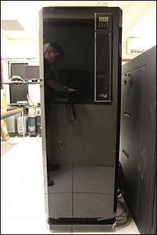
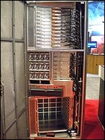
The 6600 achieved speed acceleration by outsourcing mundane work to associated computing peripherals, thus freeing up the CPU for actual data processing. The machine used the Minnesota FORTRAN compiler designed by Liddiard and Mundstock (both men were affiliated with the University of Minnesota). The compiler allowed the processor to operate at a sustained 500 kiloflops, or 0.5 megaflops, on sustained mathematical operations. The subsequent CDC7600 machine regained the mantle as the world's apex machine in 1968; it ran at 36.4 MHz (approximately 3.5 times faster than the 6600). The speed gain was achieved by using other technical innovations. Only 50 of the 7,600 machines were sold. The 7600 is depicted following:
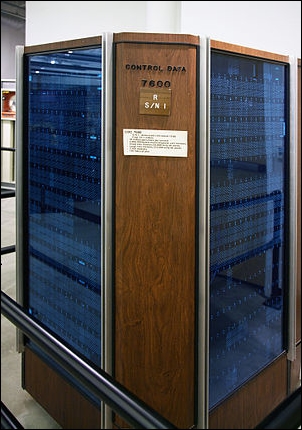
CDC7600 serial number 1 (this figure shows two sides of the C-shaped chassis)
In 1972, Cray separated from CDC to embark on a new venture. However, two years after his departure from the company, CDC introduced the STAR-100, a computational behemoth at the time, capable of executing 100 megaflops of processing power. The Texas Instruments ASC machine was also a member of this computer family. These machines ushered in what's now known as vector processing, an idea inspired by the APL programming language of the 1960s.
In 1956, researchers at Manchester University in Great Britain began experimenting with MUSE, which was derived from microsecond engine. The goal was to design a computer that could achieve processing speeds in the realm of microsecond per instruction, approximately 1 million instructions per second. At the tail end of 1958, the British electrical engineering company Ferranti collaborated with Manchester University on the MUSE project that ultimately resulted in a computer named Atlas; see the following figure:
The University of Manchester Atlas in January 1963
Atlas was commissioned on December 7, 1962, approximately three years before the CDC 6600 made its appearance as the world's first supercomputer. At that time, the Atlas was the most powerful computer in England and, some might argue, the world, having a processing capacity of four IBM 7094s, about 2 MHz. Indeed, a common refrain then was that half of Britain's computing capacity would have been lost had Atlas gone offline at any time.
Additionally, Atlas ushered in the use of virtual memory and paging - technologies used to extend its memory. The Atlas technology also gave birth to the Atlas Supervisor, which was the Windows or MAC OS of the day.
The mid-1970s and 1980s are considered the Cray era. In 1976, Cray introduced the 80 MHz Cray-1. The machine affirmatively established itself as the most successful supercomputer in history. Cray engineers incorporated integrated circuits (with two gates per chip) into the computer architecture. The chips were also capable of vector processing, which introduced innovations such as chaining, a process whereby scalar and vector registers produce a short-term result, which is then immediately used, thus obviating additional memory references, which tends to lower processing speeds. In 1982, the 105 MHz Cray X-MP was introduced. The machine boasts a shared-memory parallel vector processor with enhanced chaining support, and multiple memory pipelines. The X-MP's three floating point pipelines execute simultaneously. In 1985, the Cray-2 (see the following figure) was introduced. It had four liquid cooled processors that were fully submerged in Fluorinert, which boiled during normal operation, as heat was removed from the processors via evaporative cooling:
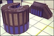
A liquid-cooled Cray-2 Supercomputer
The Cray-2 processors ran at 1.9 gigaflops, but played a subordinate role to the record holder, the Soviet Union's M-13, which operated at 2.4 gigaflops; see the following figure:

M13 Supercomputer, 1984
The M13 was dethroned in 1990 by the 10-gigaflop ETA-10G, courtesy of CDC. See the following figure:

CDC, ETA-10G Supercomputer
The 1990s saw the growth of massively parallel computing. Leading the charge was the Fujitsu Numerical Wind Tunnel supercomputer. The machine had 166 vector processors that propelled it to the apex of computational prowess in 1994. Each of the 166 processors operated at 1.7 gigaflops. However, the Hitachi SR2201, which had a distributed memory parallel system, bested the Fujitsu machine by chiming in at 614 gigaflops in 1996. The SR2201 used 2,048 processors that were linked together by a fast three-dimensional crossbar network.
The Intel Paragon, which was a contemporary of the SR2201, had 4,000 Intel i860 processors in varied configuration, and was considered the premier machine, with lineage dating back to 1993. Additionally, the Paragon used Multiple Instructions Multiple Data (MIMD) architecture, which linked processors together by way of a fast two-dimensional mesh. This configuration allows processes to run on multiple nodes (see the Appendix), using MPI. The Intel Paragon XP-E is shown here:
Intel Paragon XP-E single cabinet system Cats
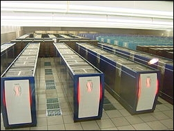
The progeny of the Paragon architecture was the intel ASCI Red supercomputer (see the following figure). Advanced Simulation and Computing Initiative (ASIC). The Red was installed at the Sandia National Laboratories in 1996, to help maintain the United States' nuclear arsenal pursuant to the 1992 memorandum on nuclear testing. The computer occupied the top spot of supercomputing machines through the end of the 20th century. The computer was massively parallel, bristling with over 9,000 computing nodes, and had more than 12 terabytes of data storage. The machine incorporated off-the-shelf Pentium Pro processors that had widely inhabited personal computers of the era. This computer punched through the 1 teraflop benchmark, ultimately reaching the new 2 teraflops benchmark:

ASCI Red supercomputer
Human desire for greater computing power entered the 21st century unabated. Petascale computing has now become the norm. A petaflop is 1 quadrillion floating point operations per second, which is 1,000 teraflops, which is 1,000,000,000,000,000 floating point operations per second, or  flops. What?! Is there an end somewhere to this madness? It should be noted that greater computing capacity usually means greater consumption of energy, which translates to greater stress on the environment. The Cray C90, which debuted in 1991, consumed 500 kilowatts of power. The ASCI Q gobbled down 3,000 kW and was 2,000 times faster than the C90 a 300-fold performance per watt increase. Oh well!
In 2004, NEC's Earth Simulator supercomputer (see the following figure) achieved 35.9 teraflops, or  flops, that is,
  flops, using 640 nodes:
NEC Earth Simulator
IBM's contribution to the teraflop genre was the Blue Gene supercomputer (see the following figure):
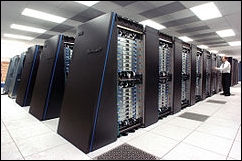
Blue Gene/P supercomputer at Argonne National Laboratory
The Blue Gene supercomputer debuted in 2007, and operated at 478.2 teraflops. Its architecture was widely used in the former part of the 21st century. Blue Gene is, essentially, an IBM project whose mission was to design supercomputers with an operating speed in the realm of petaflops, but consuming relatively low power. At first glance, this might seem an oxymoron, but IBM achieved this by employing large numbers of low-speed processors that can then be air-cooled. This computational beast uses more than 60,000 processors, which are stacked 2,048 processors per rack. The racks are interconnected in a three-dimensional torus lattice. The IBM Roadrunner maxed out at 1.105 petaflops.
China has seen rapid progress in supercomputing technology. In June 2003, China placed 51st on the TOP500 list. This list is a worldwide ranking of the world's 500 fastest supercomputers. In November 2003, China moved up the ranks to 14th place. In June 2004, it moved to fifth place, ultimately attaining first place in 2010 with the Tianhe-1 supercomputer. The machine operated at 2.56 petaflops. Then, in July 2011, the Japanese K computer achieved 10.51 petaflops, thereby attaining the top spot. The machine employed over 60,000 SPARC64 V111fx processors encased in over 600 cabinets. In 2012, the IBM Sequoia came online, operating at 16.32 petaflops. The machine's residence is the Lawrence Livermore National Laboratory, California, USA. In the same year, the Cray Titan clocked in at 17.59 petaflops. This machine resides at the Oak Ridge National Laboratory, Tennessee, USA. Then, in 2013, the Chinese unveiled the NUDT Tianhe-2 supercomputer, which had a clock speed of 33.86 petaflops, and in 2016, the Sunway TaihuLight supercomputer came online in Wuxi, China. This machine now sits atop the heap with a processing speed of 93 petaflops. This latest achievement, however, must be considered fleeting, as historical trends dictate that more powerful machines are waiting in the wings to emerge soon. Case in point, on July 29, 2015, President Obama issued an executive order to build a super machine that will clock in at a whopping 1,000 petaflops, or one exaflop, approximately 30 times faster than Tianhe-2, and approximately 10 times faster than the newly minted Sunway TaihuLight supercomputer. Stay tuned, the race continues. The following figures show the five fastest machines on the planet to date. These images are presented in ascending order of processing speed, starting with the K computer. The following figure depicts the fifth fastest supercomputer, the K computer:
K computer
The following figure depicts the fourth fastest supercomputer, the IBM Sequoia:
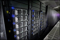
IBM Sequoia
The following figure depicts the third fastest supercomputer, the Cray Titan:
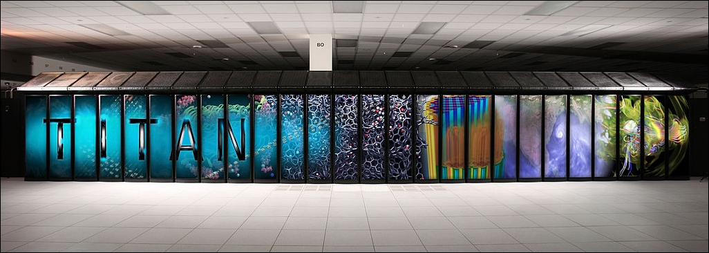
Cray Titan
The following figure depicts the second fastest supercomputer, the Tianhe-2:
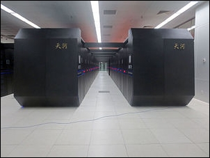
NUDT Tianhe-2
The following figure depicts the fastest supercomputer, the Sunway TaihuLight:
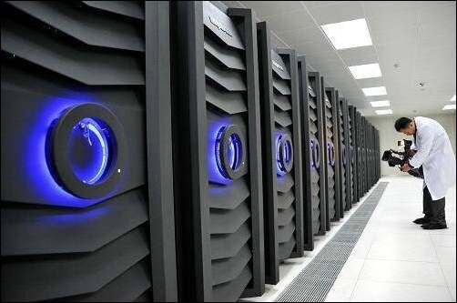
Sunway TaihuLight
Now, you might be asking yourself, so what is the process behind parallel computing? We briefly touched on this topic earlier, but now we will dig a little deeper. Let's examine the following figures, which should help you understand the mechanics behind parallel processing. We begin with the mechanics of serial processing.
The following figure shows a typical/traditional serial processing sequence:

General serial processing
Serial computing traditionally involves the following:
Breaking up the problem into chunks of instructions
Sequentially executing the instructions
Using a single processor to execute the instructions
Executing the instructions one at a time
The following figure shows an actual application of serial computing. In this case, the payroll is being processed:
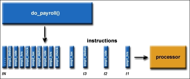
Example of payroll serial processing
The following figure shows a typical sequence in parallel processing, where there is simultaneous use of multiple compute resources employed to solve a given problem:
General parallel processing
Parallel computing involves the following:
Breaking up the problem into portions that can be concurrently solved
Breaking down each portion into a sequence of instruction sets
Simultaneously executing each portion's instruction sets on multiple processors
Using an overarching control/coordination scheme
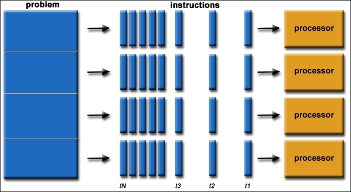
The following figure shows an actual application of parallel computing wherein the payroll is being processed:
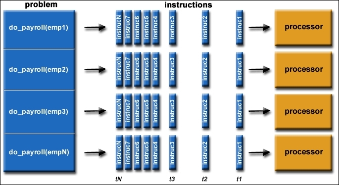
Example payroll parallel processing
One thing to note is that a given computational problem must be able to do the following:
Be broken into smaller discrete chunks to be solved simultaneously
Execute several program instructions at any given moment
Be solved in a smaller time period, employing many compute resources, as compared to using a lone compute resource
Compute resources usually consist of the following:
A sole computer possesses several processors or cores
Any number of computers/processors linked together via a network
Modern computers contain processors with multiple cores (see Appendix), typically four cores (some processors have up to 18 cores, such as the IBM BG/Q Compute Chip), making it possible to run a parallel program using MPI on a single computer/PC or node - if it is part of a supercomputer cluster (see Appendix). This one-node supercomputing capability will be explored later in the book when you are instructed on running a simple parallelized  code. These processor cores also have several functional units, such as L1 cache, L2 cache, prefetch, branch, floating-point, decode, integer, graphics processing (GPU), and so on. The following figure shows a typical supercomputing cluster (see Appendix) network:
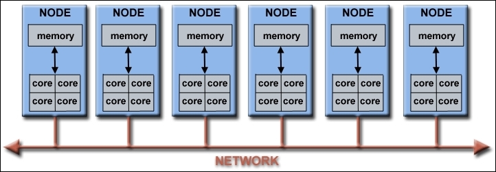
Example of a typical supercomputing network
These clusters can comprise several thousand nodes. The Blue Gene supercomputer discussed earlier has over 60,000 processors. The diminutive Raspberry Pi supercomputer has eight nodes comprising 32 cores (4 cores per Pi), or 16 nodes comprising 64 cores of processing capability. Since each node provides 4 GHz (4.8 GHz for Pi3) of processing power, your machine possesses 32 GHz ( ) or (76.8 GHz for Pi3) of processing capacity. One can argue that this little machine is indeed superior to some supercomputers of yesteryear. At this point, it should be obvious why the technique of parallel processing is superior, in most instances, to serial computing.