Logistic activation functions and classifiers

Now that the value of each location of L = {l₁, l₂, l₃, l₄, l₅, l₆} contains its availability in a vector, the locations can be sorted from the most available to the least available location. From there, the reward matrix, R, for the MDP process described in Chapter 1, Getting Started with Next-Generation Artifcial Intelligence through Reinforcement Learning, can be built.

Overall architecture

At this point, the overall architecture contains two main components:

1. Chapter 1: A reinforcement learning program based on the value-action Q function using a reward matrix that will be finalized in this chapter. The reward matrix was provided in the first chapter as an experiment, but in the implementation phase, you'll often have to build it from scratch. It sometimes takes weeks to produce a good reward matrix.
2. Chapter 2: Designing a set of 6×1 neurons that represents the flow of products at a given time at six locations. The output is the availability probability from 0 to 1. The highest value indicates the highest availability. The lowest value indicates the lowest availability.

At this point, there is some real-life information we can draw from these two main functions through an example:

• An AGV is automatically moving in a warehouse and is waiting to receive its next location to use an MDP, to calculate the optimal trajectory of its mission.
• An AGV is using a reward matrix, R, that was given during the experimental phase but needed to be designed during the implementation process.
• A system of six neurons, one per location, weighing the real quantities and probable quantities to give an availability vector, l_v, has been calculated. It is almost ready to provide the necessary reward matrix for the AGV.

To calculate the input values of the reward matrix in this reinforcement learning warehouse model, a bridge function between l_v and the reward matrix, R, is missing.

That bridge function is a logistic classifier based on the outputs of the n neurons that all perform the same tasks independently or recursively with one neuron.

At this point, the system:

• Took corporate data
• Used n neurons calculated with weights
• Applied an activation function

The activation function in this model requires a logistic classifier, a commonly used one.

Logistic classifier

The logistic classifier will be applied to l_v (the six location values) to find the best location for the AGV. This method can be applied to any other domain. It is based on the output of the six neurons as follows:

input × weight + bias

What are logistic functions? The goal of a logistic classifier is to produce a probability distribution from 0 to 1 for each value of the output vector. As you have seen so far, artificial intelligence applications use applied mathematics with probable values, not raw outputs.

The main reason is that machine learning/deep learning works best with standardization and normalization for workable homogeneous data distributions. Otherwise, the algorithms will often produce underfitted or overfitted results.

In the warehouse model, for example, the AGV needs to choose the best, most probable location, l_i. Even in a well-organized corporate warehouse, many uncertainties (late arrivals, product defects, or some unplanned problems) reduce the probability of a choice. A probability represents a value between 0 (low probability) and 1 (high probability). Logistic functions provide the tools to convert all numbers into probabilities between 0 and 1 to normalize data.

Logistic function

The logistic sigmoid provides one of the best ways to normalize the weight of a given output. The activation function of the neuron will be the logistic sigmoid. The threshold is usually a value above which the neuron has a y = 1 value; or else it has a y = 0 value. In this model, the minimum value will be 0.

The logistic function is represented as follows:

• e represents Euler's number, or 2.71828, the natural logarithm.
• x is the value to be calculated. In this case, s is the result of the logistic sigmoid function.

The code has been rearranged in the following example to show the reasoning process that produces the output, y, of the neuron:

    y1=np.multiply(x,W)+b
    y1=np.sum(y1)
    y = 1 / (1 + np.exp(-y1)) #logistic Sigmoid

Thanks to the logistic sigmoid function, the value for the first location in the model comes out squashed between 0 and 1 as 0.99, indicating a high probability that this location will be full.

To calculate the availability of the location once the 0.99 value has been taken into account, we subtract the load from the total availability, which is 1, as follows:

Availability = 1 – probability of being full (value)

Or

availability = 1 – value

As seen previously, once all locations are calculated in this manner, a final availability vector, l_v, is obtained.

When analyzing l_v, a problem has stopped the process. Individually, each line appears to be fine. By applying the logistic sigmoid to each output weight and subtracting it from 1, each location displays a probable availability between 0 and 1. However, the sum of the lines in l_v exceeds 1. That is not possible. A probability cannot exceed 1. The program needs to fix that.

Each line produces a [0, 1] solution, which fits the prerequisite of being a valid probability.

In this case, the vector l_v contains more than one value and becomes a probability distribution. The sum of l_v cannot exceed 1 and needs to be normalized.

The softmax function provides an excellent method to normalize l_v. Softmax is widely used in machine learning and deep learning.

Bear in mind that mathematical tools are not rules. You can adapt them to your problem as much as you wish as long as your solution works.

Softmax

The softmax function appears in many artificial intelligence models to normalize data. Softmax can be used for classification purposes and regression. In our example, we will use it to find an optimized goal for an MDP.

In the case of the warehouse example, an AGV needs to make a probable choice between six locations in the l_v vector. However, the total of the l_v values exceeds 1. l_v requires normalization of the softmax function, S. In the source code, the l_v vector will be named y.

The following code used is SOFTMAX.py.

1. y represents the l_v vector:

   # y is the vector of the scores of the lv vector in the warehouse example:
   y = [0.0002, 0.2, 0.9,0.0001,0.4,0.6]
   

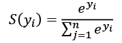
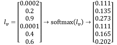
2. is the exp(i) result of each value in y (l_v in the warehouse example), as follows:

   y_exp = [math.exp(i) for i in y]
   

3. is the sum of as shown in the following code:

   sum_exp_yi = sum(y_exp)
   

Now, each value of the vector is normalized by applying the following function:

softmax = [round(i / sum_exp_yi, 3) for i in y_exp]

softmax(l_v) provides a normalized vector with a sum equal to 1, as shown in this compressed version of the code. The vector obtained is often described as containing logits.

The following code shows one version of a softmax function:

def softmax(x):
    return np.exp(x) / np.sum(np.exp(x), axis=0)

l_v is now normalized by softmax(l_v) as follows.

The last part of the softmax function requires softmax(l_v) to be rounded to 0 or 1. The higher the value in softmax(l_v), the more probable it will be. In clear-cut transformations, the highest value will be close to 1, and the others will be closer to 0. In a decision-making process, the highest value needs to be established as follows:

print("7C.
Finding the highest value in the normalized y vector : ",ohot)

The output value is 0.273 and has been chosen as the most probable location. It is then set to 1, and the other, lower values are set to 0. This is called a one-hot function. This one-hot function is extremely helpful for encoding the data provided. The vector obtained can now be applied to the reward matrix. The value 1 probability will become 100 in the R reward matrix, as follows:

The softmax function is now complete. Location l₃ or C is the best solution for the AGV. The probability value is multiplied by 100, and the reward matrix, R, can now receive the input.

We now have the data for the reward matrix. The best way to understand the mathematical aspect of the project is to draw the result on a piece of paper using the actual warehouse layout from locations A to F.

Locations={l1-A, l2-B, l3-C, l4-D, l5-E, l6-F}

Line C of the reward matrix ={0, 0, 100, 0, 0, 0}, where C (the third value) is now the target for the self-driving vehicle, in this case, an AGV in a warehouse.

Figure 2.3: Illustration of a warehouse transport problem

We obtain the following reward matrix, R, described in Chapter 1, Getting Started with Next-Generation Artificial Intelligence through Reinforcement Learning:

This reward matrix is exactly the one used in the Python reinforcement learning program using the Q function from Chapter 1. The output of this chapter is thus the input of the R matrix. The 0 values are there for the agent to avoid those values. The 1 values indicate the reachable cells. The 100 in the C×C cell is the result of the softmax output. This program is designed to stay close to probability standards with positive values, as shown in the following R matrix taken from the mdp01.py of Chapter 1:

R = ql.matrix([ [0,0,0,0,1,0],
                [0,0,0,1,0,1],
                [0,0,100,1,0,0],
                [0,1,1,0,1,0],
                [1,0,0,1,0,0],
                [0,1,0,0,0,0] ])

At this point:

• The output of the functions in this chapter generated a reward matrix, R, which is the input of the MDP described in Chapter 1, Getting Started with Next-Generation Artificial Intelligence through Reinforcement Learning.
• The MDP process was set to run for 50,000 episodes in Chapter 1.
• The output of the MDP has multiple uses, as we saw in this chapter and Chapter 1.

The building blocks are in place to begin evaluating the execution and performances of the reinforcement learning program, as we will see in Chapter 3, Machine Intelligence – Evaluation Functions and Numerical Convergence.