-
Book Overview & Buying
-
Table Of Contents

GNU Octave Beginner's Guide
By :
GNU Octave Beginner's Guide
By:
Overview of this book
Today, scientific computing and data analysis play an integral part in most scientific disciplines ranging from mathematics and biology to imaging processing and finance. With GNU Octave you have a highly flexible tool that can solve a vast number of such different problems as complex statistical analysis and dynamical system studies.The GNU Octave Beginner's Guide gives you an introduction that enables you to solve and analyze complicated numerical problems. The book is based on numerous concrete examples and at the end of each chapter you will find exercises to test your knowledge. It's easy to learn GNU Octave, with the GNU Octave Beginner's Guide to hand.Using real-world examples the GNU Octave Beginner's Guide will take you through the most important aspects of GNU Octave. This practical guide takes you from the basics where you are introduced to the interpreter to a more advanced level where you will learn how to build your own specialized and highly optimized GNU Octave toolbox package. The book starts by introducing you to work variables like vectors and matrices, demonstrating how to perform simple arithmetic operations on these objects before explaining how to use some of the simple functionality that comes with GNU Octave, including plotting. It then goes on to show you how to write new functionality into GNU Octave and how to make a toolbox package to solve your specific problem. Finally, it demonstrates how to optimize your code and link GNU Octave with C and C++ code enabling you to solve even the most computationally demanding tasks. After reading GNU Octave Beginner's Guide you will be able to use and tailor GNU Octave to solve most numerical problems and perform complicated data analysis with ease.
Table of Contents (11 chapters)
Preface

 Free Chapter
1. Introducing GNU Octave
2. Interacting with Octave: Variables and Operators
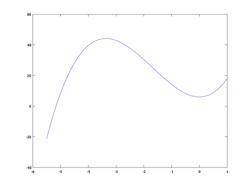
3. Working with Octave:Functions and Plotting
4. Rationalizing: Octave Scripts
5. Extensions: Write Your Own Octave Functions
6. Making Your Own Package: A Poisson Equation Solver
7. More Examples: Data Analysis
8. Need for Speed: Optimization and Dynamically Linked Functions
A. Pop Quiz Answers
Index