
In the previous section, we saw what a write concern is and how it affects the write operations (insert, update, and delete). In this section, we will see what a read preference is and how it affects query operations. We'll discuss how to use a read preference in separate recipes, to use specific programming language drivers.
When connected to an individual node, query operations will be allowed by default when connected to a primary, and in case if it is connected to a secondary node, we need to explicitly state that it is ok to query from secondary instances by executing rs.slaveOk() from the shell.
However, consider connecting to a Mongo replica set from an application. It will connect to the replica set and not a single instance from the application. Depending on the nature of the application, it might always want to connect to a primary; always to a secondary; prefer connecting to a primary node but would be ok to connect to a secondary node in some scenarios and vice versa and finally, it might connect to the instance geographically close to it (well, most of the time).
Thus, the read preference plays an important role when connected to a replica set and not to a single instance. In the following table, we will see the various read preferences that are available and what their behavior is in terms of querying a replica set. There are five of them and the names are self-explanatory:
Similar to how write concerns can be coupled with shard tags, read preferences can also be used along with shard tags. As the concept of tags has already been introduced in Chapter 4, Administration, you can refer to it for more details.
We just saw what the different types of read preferences are (except for those using tags) but the question is, how do we use them? We have covered Python and Java clients in this book and will see how to use them in their respective recipes. We can set read preferences at various levels: at the client level, collection level, and query level, with the one specified at the query level overriding any other read preference set previously.
Let us see what the nearest read preference means. Conceptually, it can be visualized as something like the following diagram:
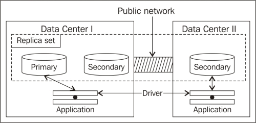
A Mongo replica set is set up with one secondary, which can never be a primary, in a separate data center and two (one primary and a secondary) in another data center. An identical application deployed in both the data centers, with a primary read preference, will always connect to the primary instance in Data Center I. This means, for the application in Data Center II, the traffic goes over the public network, which will have high latency. However, if the application is ok with slightly stale data, it can set the read preference as the nearest, which will automatically let the application in Data Center I connect to an instance in Data Center I and will allow an application in Data Center II to connect to the secondary instance in Data Center II.
But then the next question is, how does the driver know which one is the nearest? The term "geographically close" is misleading; it is actually the one with the minimum network latency. The instance we query might be geographically further than another instance in the replica set, but it can be chosen just because it has an acceptable response time. Generally, better response time means geographically closer.
The following section is for those interested in internal details from the driver on how the nearest node is chosen. If you are happy with just the concepts and not the internal details, you can safely skip the rest of the contents.
Let us see some pieces of code from a Java client (driver 2.11.3 is used for this purpose) and make some sense out of it. If we look at the com.mongodb.TaggableReadPreference.NearestReadPreference.getNode method, we see the following implementation:
@Override
ReplicaSetStatus.ReplicaSetNode getNode(ReplicaSetStatus.ReplicaSet set) {
  if (_tags.isEmpty())
    return set.getAMember();

  for (DBObject curTagSet : _tags) {
    List<ReplicaSetStatus.Tag> tagList = getTagListFromDBObject(curTagSet);
    ReplicaSetStatus.ReplicaSetNode node = set.getAMember(tagList);
    if (node != null) {
      return node;
    }
  }
  return null;
}
For now, if we ignore the contents where tags are specified, all it does is execute set.getAMember().
The name of this method tells us that there is a set of replica set members and we returned one of them randomly. Then what decides whether the set contains a member or not? If we dig a bit further into this method, we see the following lines of code in the com.mongodb.ReplicaSetStatus.ReplicaSet class:
public ReplicaSetNode getAMember() {
  checkStatus();
  if (acceptableMembers.isEmpty()) {
    return null;
  }
  return acceptableMembers.get(random.nextInt(acceptableMembers.size()));
}
Ok, so all it does is pick one from a list of replica set nodes maintained internally. Now, the random pick can be a secondary, even if a primary can be chosen (because it is present in the list). Thus, we can now say that when the nearest is chosen as a read preference, and even if a primary is in the list of contenders, it might not necessarily be chosen randomly.
The question now is, how is the acceptableMembers list initialized? We see it is done in the constructor of the com.mongodb.ReplicaSetStatus.ReplicaSet class as follows:
this.acceptableMembers =Collections.unmodifiableList(calculateGoodMembers(all, calculateBestPingTime(all, true),acceptableLatencyMS, true));
The calculateBestPingTime line just finds the best ping time of all (we will see what this ping time is later).
Another parameter worth mentioning is acceptableLatencyMS. This gets initialized in com.mongodb.ReplicaSetStatus.Updater (this is actually a background thread that updates the status of the replica set continuously), and the value for acceptableLatencyMS is initialized as follows:
slaveAcceptableLatencyMS = Integer.parseInt(System.getProperty("com.mongodb.slaveAcceptableLatencyMS", "15"));As we can see, this code searches for the system variable called com.mongodb.slaveAcceptableLatencyMS, and if none is found, it initializes to the value 15, which is 15 ms.
This com.mongodb.ReplicaSetStatus.Updater class also has a run method that periodically updates the replica set stats. Without getting too much into it, we can see that it calls updateAll, which eventually reaches the update method in com.mongodb.ConnectionStatus.UpdatableNode:
long start = System.nanoTime();
CommandResult res = _port.runCommand(_mongo.getDB("admin"), isMasterCmd);
long end = System.nanoTime()
All it does is execute the {isMaster:1} command and record the response time in nanoseconds. This response time is converted to milliseconds and stored as the ping time. So, coming back to the com.mongodb.ReplicaSetStatus.ReplicaSet class it stores, all calculateGoodMembers does is find and add the members of a replica set that are no more than acceptableLatencyMS milliseconds more than the best ping time found in the replica set.
For example, in a replica set with three nodes, the ping times from the client to the three nodes (node 1, node 2, and node 3) are 2 ms, 5 ms, and 150 ms respectively. As we see, the best time is 2 ms and hence, node 1 goes into the set of good members. Now, from the remaining nodes, all those with a latency that is no more than acceptableLatencyMS more than the best, which is 2 + 15 ms = 17 ms, as 15 ms is the default that will be considered. Thus, node 2 is also a contender, leaving out node 3. We now have two nodes in the list of good members (good in terms of latency).
Now, putting together all that we saw on how it would work for the scenario we saw in the preceding diagram, the least response time will be from one of the instances in the same data center (from the programming language driver's perspective in these two data centers), as the instance(s) in other data centers might not respond within 15 ms (the default acceptable value) more than the best response time due to public network latency. Thus, the acceptable nodes in Data Center I will be two of the replica set nodes in that data center, and one of them will be chosen at random, and for Data Center II, only one instance is present and is the only option. Hence, it will be chosen by the application running in that data center.