One of the cases when the tabular CPD isn't a good choice is when we have a deterministic random variable, whose value depends only on the values of its parents in the model. For such a variable X with parents Par(X), we have the following:

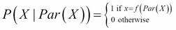
Here, .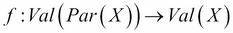

We can take the example of logic gates (AND, OR, and so on), where the output of the gate is deterministic in nature and depends only on its inputs. We represent it as a Bayesian network, as shown in Fig 1.7:

Fig 1.7: A Bayesian network for a logic gate. X and Y are the inputs, A and B are the outputs and Z is a deterministic variable representing the operation of the logic gate.

Here, X and Y are the inputs to the logic gate and Z is the output. We usually denote a deterministic variable by double circles. We can also see that having a deterministic variable gives up more information about the independencies in the network. If we are given the values of X and Y, we know the value of Z, which leads us to the assertion .

We saw the case of deterministic variables where there was a structure in the CPD, which can help us reduce the size of the whole CPD table. As in the case of deterministic variables, structure may occur in many other problems as well. Think of adding a variable Flat Tyre to our late-for-school model. If we have a Flat Tyre (F), irrespective of the values of all other variables, the value of the Late for school variable is always going to be 1. If we think of representing this situation using a tabular CPD, we will have all the values for Late for school corresponding to F = 1 that will be 1, which would essentially be half the table. Hence, if we use tabular CPD, we will be wasting a lot of memory to store values that can simply be represented by a single condition. In such cases, we can use the Tree CPD or Rule CPD.

Tree CPD

A great option to represent such context-specific cases is to use a tree structure to represent the various contexts. In a Tree CPD, each leaf represents the various possible conditional distributions, and the path to the leaf represents the conditions for that distribution. Let's take an example by adding a Flat Tyre variable to our earlier model, as shown in Fig 1.8:

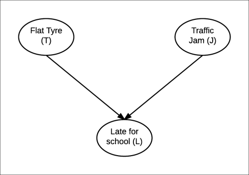
Fig 1.8: Network after adding Flat Tyre (T) variable

If we represent the CPD of L using a Tree CPD, we will get something like this:

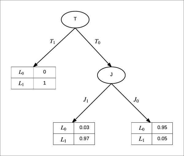
Fig 1.9: Tree CPD in case of Flat tyre

Here, we can see that rather than having four values for the CPD, which we would have to store in the case of Tabular CPD, we only need to store three values in the case of the Tree CPD. This improvement doesn't seem very significant right now, but when we have a large number of variables with high cardinalities, there is a very significant improvement.

Now, let's see how we can implement this using pmgpy:

In [1]: from pgmpy.factors import TreeCPD, Factor
In [2]: tree_cpd = TreeCPD([
                   ('B', Factor(['A'], [2], [0.8, 0.2]), '0'),
                   ('B', 'C', '1'),
                   ('C', Factor(['A'], [2], [0.1, 0.9]), '0'),
                   ('C', 'D', '1'),
                   ('D', Factor(['A'], [2], [0.9, 0.1]), '0'),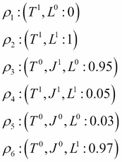
                   ('D', Factor(['A'], [2], [0.4, 0.6]), '1')])

Note

pgmpy also supports Tree CPDs, where each node has more than one variable.

Rule CPD

Rule CPD is another more explicit form of representation of CPDs. Rule CPD is basically a set of rules along with the corresponding values of the variable. Taking the same example of Flat Tyre, we get the following Rule CPD:

Let's see the code implementation using pgmpy:

In [1]: from pgmpy.factors import RuleCPD
In [2]: rule = RuleCPD('A', {('A_0', 'B_0'): 0.8,
                             ('A_1', 'B_0'): 0.2,
                             ('A_0', 'B_1', 'C_0'): 0.4,
                             ('A_1', 'B_1', 'C_0'): 0.6,
                             ('A_0', 'B_1', 'C_1'): 0.9,
                             ('A_1', 'B_1', 'C_1'): 0.1})